Partial Differential Equations

1. Partial Differential Equations • Introduction, Adam Zornes • Discretizations and Iterative Solvers, Chenfang Chen • Parallelization, Dr. Danny Thorne

2. What do You Stand For? • A PDE is a Partial Differential Equation • This is an equation with derivatives of at least two variables in it. • In general, partial differential equations are much more difficult to solve analytically than are ordinary differential equations

3. What Does a PDE Look Like • Let u be a function of x and y. There are several ways to write a PDE, e.g., • ux + uy = 0 • du/dx + du/dy = 0

4. The Baskin Robin’s esq Characterization of PDE’s • The order is determined by the maximum number of derivatives of any term. • Linear/Nonlinear • A nonlinear PDE has the solution times a partial derivative or a partial derivative raised to some power in it • Elliptic/Parabolic/Hyperbolic

5. Six One Way • Say we have the following: Auxx + 2Buxy + Cuyy + Dux + Euy + F = 0. • Look at B2 - AC • < 0 elliptic • = 0 parabolic • > 0 hyperbolic

6. Or Half a Dozen Another • A general linear PDE of order 2: • Assume symmetry in coefficients so that A = [aij] is symmetric. Eig(A) are real. Let P and Z denote the number of positive and zero eigenvalues of A. • Elliptic: Z = 0 and P = n or Z = 0 and P = 0.. • Parabolic: Z > 0 (det(A) = 0). • Hyperbolic: Z=0 and P = 1 or Z = 0 and P = n-1. • Ultra hyperbolic: Z = 0 and 1 < P < n-1.

7. Elliptic, Not Just For Exercise Anymore • Elliptic partial differential equations have applications in almost all areas of mathematics, from harmonic analysis to geometry to Lie theory, as well as numerous applications in physics. • The basic example of an elliptic partial differential equation is Laplace’s Equation • uxx - uyy = 0

8. The Others • The heat equation is the basic Hyperbolic • ut - uxx - uyy = 0 • The wave equations are the basic Parabolic • ut - ux - uy = 0 • utt - uxx - uyy = 0 • Theoretically, all problems can be mapped to one of these

9. What Happens Where You Can’t Tell What Will Happen • Types of boundary conditions • Dirichlet: specify the value of the function on a surface • Neumann: specify the normal derivative of the function on a surface • Robin: a linear combination of both • Initial Conditions

10. Is It Worth the Effort? • Basically, is it well-posed? • A solution to the problem exists. • The solution is unique. • The solution depends continuously on the problem data. • In practice, this usually involves correctly specifying the boundary conditions

11. Why Should You Stay Awake for the Remainder of the Talk? • Enormous application to computational science, reaching into almost every nook and cranny of the field including, but not limited to: physics, chemistry, etc.

12. Example • Laplace’s equation involves a steady state in systems of electric or magnetic fields in a vacuum or the steady flow of incompressible non-viscous fluids • Poisson’s equation is a variation of Laplace when an outside force is applied to the system

13. Poisson Equation in 2D

14. Example: CFD

15. Computational Fluid Dynamics • CFD can be defined narrowly as confined to aerodynamic flow around vehicles but it can be generalized to include as well such areas as weather and climate simulation, flow of pollutants in the earth, and flow of liquids in oil fields (reservoir modelling). • Involve Huge PDE’s • Computational Science only Realistic Solution

16. Links • http://www.npac.syr.edu/users/gcf/cps713overI94/ • http://www.cse.uiuc.edu/~rjhartma/pdesong.html • http://www.maths.soton.ac.uk/teaching/units/ma274/node2.html • http://www.npac.syr.edu/projects/csep/pde/pde.html • http://mathworld.wolfram.com/PartialDifferentialEquation.html

17. Discretization and Iterative Method for PDEs Chunfang Chen Danny Thorne Adam Zornes

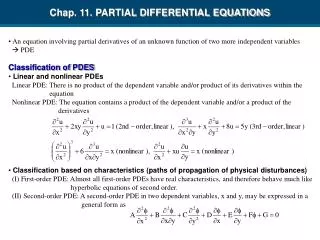
18. Classification of PDEs Different mathematical and physical behaviors: • Elliptic Type • Parabolic Type • Hyperbolic Type System of coupled equations for several variables: • Time : first-derivative (second-derivative for wave equation) • Space: first- and second-derivatives

19. Classification of PDEs (cont.) General form of second-order PDEs ( 2 variables)

20. PDE Model Problems • Hyperbolic (Propagation) • Advection equation (First-order linear) • Wave equation (Second-order linear)

21. PDE Model Problems (cont.) • Parabolic (Time- or space-marching) • Burger’s equation(Second-order nonlinear) • Fourier equation (Second-order linear) (Diffusion / dispersion)

22. PDE Model Problems (cont.) • Elliptic (Diffusion, equilibrium problems) • Laplace/Poisson (second-order linear) • Helmholtz equation (second-order linear)

23. PDE Model Problems (cont.) • System of Coupled PDEs • Navier-Stokes Equations

24. Well-Posed Problem Numerically well-posed • Discretization equations • Auxiliary conditions (discretized approximated) • the computational solution exists (existence) • the computational solution is unique (uniqueness) • the computational solution depends continuously on the approximate auxiliary data • the algorithm should be well-posed (stable) also

25. Boundary and InitialConditions R • Initial conditions:starting point for propagation problems • Boundary conditions:specified on domain boundaries to provide the interior solution in computational domain R s n

26. Numerical Methods • Complex geometry • Complex equations (nonlinear, coupled) • Complex initial / boundary conditions • No analytic solutions • Numerical methods needed !!

27. Numerical Methods Objective: Speed, Accuracy at minimum cost • Numerical Accuracy(error analysis) • Numerical Stability(stability analysis) • Numerical Efficiency (minimize cost) • Validation (model/prototype data, field data, analytic solution, theory, asymptotic solution) • Reliability and Flexibility(reduce preparation and debugging time) • Flow Visualization(graphics and animations)

28. computational solution procedures Governing Equations ICS/BCS System of Algebraic Equations Equation (Matrix) Solver ApproximateSolution Discretization Ui (x,y,z,t) p (x,y,z,t) T (x,y,z,t) or  (,,, ) Continuous Solutions Finite-Difference Finite-Volume Finite-Element Spectral Boundary Element Hybrid Discrete Nodal Values Tridiagonal ADI SOR Gauss-Seidel Krylov Multigrid DAE

29. Discretization • Time derivatives almost exclusively by finite-difference methods • Spatial derivatives - Finite-difference: Taylor-series expansion - Finite-element: low-order shape function and interpolation function, continuous within each element - Finite-volume: integral form of PDE in each control volume - There are also other methods, e.g. collocation, spectral method, spectral element, panel method, boundary element method

30. Finite Difference • Taylor series • Truncation error • How to reduce truncation errors? • Reduce grid spacing, use smaller x = x-xo • Increase order of accuracy, use larger n

31. Finite Difference Scheme • Forward difference • Backward difference • Central difference

32. y x Example : Poisson Equation (-1,1) (1,1) (-1,-1) (1,-1)

33. Example (cont.)

34. Rectangular Grid After we discretize the Poisson equation on a rectangular domain, we are left with a finite number of gird points. The boundary values of the equation are the only known grid points

35. What to solve? Discretization produces a linear system of equations. The A matrix is a pentadiagonal banded matrix of a standard form: A solution method is to be performed for solving

36. Matrix Storage We could try and take advantage of the banded nature of the system, but a more general solution is the adoption of a sparse matrix storage strategy.

37. Limitations of Finite Differences • Unfortunately, it is not easy to use finite differences in complex geometries. • While it is possible to formulate curvilinear finite difference methods, the resulting equations are usually pretty nasty.

38. Finite Element Method • The finite element method, while more complicated than finite difference methods, easily extends to complex geometries. • A simple (and short) description of the finite element method is not easy to give. Weak Form Matrix System PDE

39. Finite Element Method (Variational Formulations) • Find u in test space H such that a(u,v) = f(v) for all v in H, where a is a bilinear form and f is a linear functional. • V(x,y) = j Vjj(x,y), j = 1,…,n • I(V) = .5 j j AijViVj - j biVi, i,j = 1,…,n • Aij =  a( j,  j), i = 1,…,n • Bi =  f j, i = 1,…,n • The coefficients Vj are computed and the function V(x,y) is evaluated anyplace that a value is needed. • The basis functions should have local support (i.e., have a limited area where they are nonzero).

40. Time Stepping Methods • Standard methods are common: • Forward Euler (explicit) • Backward Euler (implicit) • Crank-Nicolson (implicit) θ = 0, Fully-Explicit θ = 1, Fully-Implicit θ = ½, Crank-Nicolson

41. Time Stepping Methods (cont.) • Variable length time stepping • Most common in Method of Lines (MOL) codes or Differential Algebraic Equation (DAE) solvers

42. Solving the System • The system may be solved using simple iterative methods - Jacobi, Gauss-Seidel, SOR, etc. • Some advantages: - No explicit storage of the matrix is required - The methods are fairly robust and reliable • Some disadvantages - Really slow (Gauss-Seidel) - Really slow (Jacobi)

43. Solving the System • Advanced iterative methods (CG, GMRES) CG is a much more powerful way to solve the problem. • Some advantages: • Easy to program (compared to other advanced methods) • Fast (theoretical convergence in N steps for an N by N system) • Some disadvantages: • Explicit representation of the matrix is probably necessary • Applies only to SPD matrices

44. Multigrid Algorithm: Components • Residual • compute the error of the approximation • Iterative method/Smoothing Operator • Gauss-Seidel iteration • Restriction • obtain a ‘coarse grid’ • Prolongation • from the ‘coarse grid’ back to the original grid

45. Residual Vector • The equation we are to solve is defined as: • So then the residual is defined to be: • Where uq is a vector approximation for u • As the u approximation becomes better, the components of the residual vector(r) , move toward zero

46. Multigrid Algorithm: Components • Residual • compute the error of your approximation • Iterative method/Smoothing Operator • Gauss-Seidel iteration • Restriction • obtain a ‘coarse grid’ • Prolongation • from the ‘coarse grid’ back to the original grid

47. Multigrid Algorithm: Components • Residual • compute the error of your approximation • Iterative method/Smoothing Operator • Gauss-Seidel iteration • Restriction • obtain a ‘coarse grid’ • Prolongation • from the ‘coarse grid’ back to the original grid

48. The Restriction Operator • Defined as ‘half-weighted’ restriction. • Each new point in the courser grid, is dependent upon it’s neighboring points from the fine grid

49. Multigrid Algorithm: Components • Residual • compute the error of your approximation • Iterative method/Smoothing Operator • Gauss-Seidel iteration • Restriction • obtain a ‘coarse grid’ • Prolongation • from the ‘coarse grid’ back to the original grid

50. The Prolongation Operator • The grid change is exactly the opposite of restriction