Download
1 / 48
690 likes | 1.7k Views
Elliptic Partial Differential Equations - Introduction. http://numericalmethods.eng.usf.edu Transforming Numerical Methods Education for STEM Undergraduates. 9/3/2014. http://numericalmethods.eng.usf.edu. 1. For more details on this topic Go to http://numericalmethods.eng.usf.edu

E N D
Elliptic Partial Differential Equations - Introduction http://numericalmethods.eng.usf.edu Transforming Numerical Methods Education for STEM Undergraduates 9/3/2014 http://numericalmethods.eng.usf.edu 1
For more details on this topic • Go to http://numericalmethods.eng.usf.edu • Click on Keyword • Click on Elliptic Partial Differential Equations
You are free • to Share – to copy, distribute, display and perform the work • to Remix – to make derivative works
Under the following conditions • Attribution — You must attribute the work in the manner specified by the author or licensor (but not in any way that suggests that they endorse you or your use of the work). • Noncommercial — You may not use this work for commercial purposes. • Share Alike — If you alter, transform, or build upon this work, you may distribute the resulting work only under the same or similar license to this one.
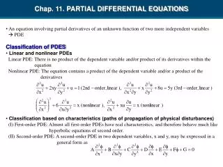
Defining Elliptic PDE’s • The general form for a second order linear PDE with two independent variables ( ) and one dependent variable ( ) is • Recall the criteria for an equation of this type to be considered elliptic • For example, examine the Laplace equation given by then thus allowing us to classify this equation as elliptic. , where , ,
Physical Example of an Elliptic PDE Schematic diagram of a plate with specified temperature boundary conditions The Laplace equation governs the temperature:
Discretizing the Elliptic PDE Substituting these approximations into the Laplace equation yields: if, the Laplace equation can be rewritten as
Discretizing the Elliptic PDE • Once the governing equation has been discretized there are several numerical methods that can be used to solve the problem. • We will examine the: • Direct Method • Gauss-Seidel Method • Lieberman Method
The End http://numericalmethods.eng.usf.edu
Acknowledgement This instructional power point brought to you by Numerical Methods for STEM undergraduate http://numericalmethods.eng.usf.edu Committed to bringing numerical methods to the undergraduate
For instructional videos on other topics, go to http://numericalmethods.eng.usf.edu/videos/ This material is based upon work supported by the National Science Foundation under Grant # 0717624. Any opinions, findings, and conclusions or recommendations expressed in this material are those of the author(s) and do not necessarily reflect the views of the National Science Foundation.
Example 1: Direct Method Consider a plate that is subjected to the boundary conditions shown below. Find the temperature at the interior nodes using a square grid with a length of by using the direct method.
Example 1: Direct Method We can discretize the plate by taking,
Example 1: Direct Method The nodal temperatures at the boundary nodes are given by:
Example 1: Direct Method Here we develop the equation for the temperature at the node (2,3) i=2 and j=3
Example 1: Direct Method We can develop similar equations for every interior node leaving us with an equal number of equations and unknowns. Question: How many equations would this generate?
Example 1: Direct Method We can develop similar equations for every interior node leaving us with an equal number of equations and unknowns. Question: How many equations would this generate? Answer: 12 Solving yields:
The Gauss-Seidel Method • Recall the discretized equation • This can be rewritten as • For the Gauss-Seidel Method, this equation is solved iteratively for all interior nodes until a pre-specified tolerance is met.
Example 2: Gauss-Seidel Method Consider a plate that is subjected to the boundary conditions shown below. Find the temperature at the interior nodes using a square grid with a length of using the Gauss-Siedel method. Assume the initial temperature at all interior nodes to be .
Example 2: Gauss-Seidel Method We can discretize the plate by taking
Example 2: Gauss-Seidel Method The nodal temperatures at the boundary nodes are given by:
Example 2: Gauss-Seidel Method • Now we can begin to solve for the temperature at each interior node using • Assume all internal nodes to have an initial temperature of zero. Iteration #1 i=1 and j=1 i=1 and j=2
Example 2: Gauss-Seidel Method After the first iteration, the temperatures are as follows. These will now be used as the nodal temperatures for the second iteration.
Example 2: Gauss-Seidel Method Iteration #2 i=1 and j=1
Example 2: Gauss-Seidel Method The figures below show the temperature distribution and absolute relative error distribution in the plate after two iterations: Absolute Relative Approximate Error Distribution Temperature Distribution
The Lieberman Method • Recall the equation used in the Gauss-Siedel Method, • Because the Guass-Siedel Method is guaranteed to converge, we can accelerate the process by using over- relaxation. In this case,
Example 3: Lieberman Method Consider a plate that is subjected to the boundary conditions shown below. Find the temperature at the interior nodes using a square grid with a length of . Use a weighting factor of 1.4 in the Lieberman method. Assume the initial temperature at all interior nodes to be .
Example 3: Lieberman Method We can discretize the plate by taking
Example 3: Lieberman Method We can also develop equations for the boundary conditions to define the temperature of the exterior nodes.
Example 3: Lieberman Method • Now we can begin to solve for the temperature at each interior node using the rewritten Laplace equation from the Gauss-Siedel method. • Once we have the temperature value for each node we will apply the over relaxation equation of the Lieberman method • Assume all internal nodes to have an initial temperature of zero. Iteration #2 Iteration #1 i=1 and j=1 i=1 and j=2
Example 3: Lieberman Method After the first iteration the temperatures are as follows. These will be used as the initial nodal temperatures during the second iteration.
Example 3: Lieberman Method Iteration #2 i=1 and j=1
Example 3: Lieberman Method The figures below show the temperature distribution and absolute relative error distribution in the plate after two iterations: Absolute Relative Approximate Error Distribution Temperature Distribution
Insulated Alternative Boundary Conditions • In Examples 1-3, the boundary conditions on the plate had a specified temperature on each edge. What if the conditions are different ? For example, what if one of the edges of the plate is insulated. • In this case, the boundary condition would be the derivative of the temperature. Because if the right edge of the plate is insulated, then the temperatures on the right edge nodes also become unknowns.
Insulated Alternative Boundary Conditions • The finite difference equation in this case for the right edge for the nodes for • However the node is not inside the plate. The derivative boundary condition needs to be used to account for these additional unknown nodal temperatures on the right edge. This is done by approximating the derivative at the edge node as
Alternative Boundary Conditions • Rearranging this approximation gives us, • We can then substitute this into the original equation gives us, • Recall that is the edge is insulated then, • Substituting this again yields,
Insulated Example 3: Alternative Boundary Conditions A plate is subjected to the temperatures and insulated boundary conditions as shown in Fig. 12. Use a square grid length of . Assume the initial temperatures at all of the interior nodes to be . Find the temperatures at the interior nodes using the direct method.
Example 3: Alternative Boundary Conditions We can discretize the plate taking,
Example 3: Alternative Boundary Conditions We can also develop equations for the boundary conditions to define the temperature of the exterior nodes. Insulated
Example 3: Alternative Boundary Conditions Here we develop the equation for the temperature at the node (4,3), to show the effects of the alternative boundary condition. i=4 and j=3
Example 3: Alternative Boundary Conditions The addition of the equations for the boundary conditions gives us a system of 16 equations with 16 unknowns. Solving yields: