Download

1 / 98
1.03k likes | 1.49k Views
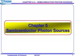
Chapter 5 Semiconductor Photon Sources. injection electroluminescence A light-emitting diode (LED) : a forward-biased p-n junction fabricated from a direct-gap semiconductor material that emits light via injection electroluminescence

E N D
Chapter 5 Semiconductor Photon Sources Fundamentals of Photonics
injection electroluminescence A light-emitting diode (LED) : a forward-biased p-n junction fabricated from a direct-gap semiconductor material that emits light via injection electroluminescence forward voltage increased beyond a certain value population inversion The junction may then be used as a diode laser amplifier or, with appropriate feedback, as an injection laser diode. Semiconductor Photon Sources Fundamentals of Photonics
Advantages: readily modulated by controlling the injected current efficiency high reliability compatibility with electronic systems Applications: lamp indicators; display devices; scanning, reading, and printing systems; fiber-optic communication systems; and optical data storage systems such as compact-disc players Semiconductor Photon Sources Fundamentals of Photonics
Injection Electroluminescence Electroluminescence in Thermal Equilibrium At room temperature the concentration of thermally excited electrons and holes is so small that the generated photon flux is very small. 16.1 LIGHT-EMITTING DIODES Fundamentals of Photonics
Electroluminescence in the Presence of Carrier Injection The photon emission rate may be calculated from the electron-hole pair injection rate R (pairs/cm3-s), where R plays the role of the laser pumping rate. Assume that the excess electron-hole pairs recombine at the rate 1/τ, where τ is the overall (radiative and nonradiative) electron-hole recombination time Fundamentals of Photonics
Electroluminescence in the Presence of Carrier Injection Under steady-state conditions, the generation (pumping) rate must precisely balance the recombination (decay) rate, so that R = ∆n/τ. Thus the steady-state excess carrier concentration is proportional to the pumping rate, i.e., (16.1-1) Fundamentals of Photonics
Electroluminescence in the Presence of Carrier Injection Only radiative recombinations generate photons, however, and the internal quantum efficiency ηi = τ/τr, accounts for the fact that only a fraction of the recombinations are radiative in nature. The injection of RV carrier pairs per second therefore leads to the generation of a photon flux Q = ηiRV photons/s, i.e., (16.1-2) Fundamentals of Photonics
Electroluminescence in the Presence of Carrier Injection The internal quantum efficiency ηi plays a crucial role in determining the performance of this electron-to-photon transducer. Direct-gap semiconductors are usually used to make LEDs (and injection lasers) because ηi is substantially larger than for indirect-gap semiconductors (e.g., ηi = 0.5 for GaAs, whereas ηi = 10-5 for Si, as shown in Table 15.1-5). The internal quantum efficiency ηi depends on the doping, temperature, and defect concentration of the material. Fundamentals of Photonics
Spectral Density of Electroluminescence Photons The spectral density of injection electroluminescence light may be determined by using the direct band-to-band emission theory developed in Sec. 15.2. The rate of spontaneous emission rsp(v) (number of photons per second per hertz per unit volume), as provided in (15.2-16), is (16.1-3) Fundamentals of Photonics
Spectral Density of Electroluminescence Photons where τr, is the radiative electron-hole recombination lifetime. The optical joint density of states for interaction with photons of frequency v, as given in (15.2-9), is where mr, is related to the effective masses of the holes and electrons by 1/ mr = 1/mv + 1/mc, [as given in (15.2-5)], and Eg is the bandgap energy. The emission condition [as given in (15.2-10)] provides (16.1-4) Fundamentals of Photonics
Spectral Density of Electroluminescence Photons which is the probability that a conduction-band state of energy is filled and a valence-band state of energy is empty, as provided in (15.26) and (15.2-7) and illustrated in Fig. 16.1-2. Equations (16.1-5) and (16.1-6) guarantee that energy and momentum are conserved. (16.1-5) (16.1-6) Fundamentals of Photonics
E2 Ec Eg Ev E1 K Figure 16.1-2 The spontaneous emission of a photon resulting from the recombination of an electron of energy E2, with a hole of energy E1=E2-hv. The transition is represented by a vertical arrow because the momentum carried away by the photon, hv/c, is negligible on the scale of the figure. Fundamentals of Photonics
Spectral Density of Electroluminescence Photons The semiconductor parameters Eg, τr, mv and mc, and the temperature T determine the spectral distribution rsp(v), given the quasi-Fermi levels Efc and Efv. These, in turn, are determined from the concentrations of electrons and holes given in (15.1-7) and (15.1-8), The densities of states near the conduction- and valence-band edges are, respectively, as per (15.1-4) and (15.1-5), (16.1-7) Fundamentals of Photonics
Spectral Density of Electroluminescence Photons Increasing the pumping level R causes ∆n to increase, which, in turn, moves Efc toward (or further into) the conduction band, and Efv toward (or further into) the valence band. This results in an increase in the probability fc(E2) of finding the conduction-band state of energy E2 filled with an electron, and the probability 1 - fv(E1) of finding the valence-band state of energy E1 empty (filled with a hole). The net result is that the emission-condition probability fe(v) = fc(E2) [1 - fv(E1) ] increases with R, thereby enhancing the spontaneous emission rate given in (16.1-3). Fundamentals of Photonics
EXERCISE 16.1- 1 Quasi-Fermi Levels of a Pumped Semiconductor. (a) Under ideal conditions at T = 0 K, when there is no thermal electron-hole pair generation [see Fig. 16.1-3(a)], show that the quasi-Fermi levels are related to the concentrations of injected electron-hole pairs ∆n by (16.1-8a) (16.1-8b) Fundamentals of Photonics
E E E E Efc Fc(E) Efc Fc(E) Efv Fv(E) Efv Fv(E) K K (b) (a) Figure 16.1-3 Energy bands and Fermi functions for a semiconductor in quasi-equilibrium (a) at T=0K, and (b) T>0K. Fundamentals of Photonics
so that where ∆n 》n0,p0. Under these conditions all ∆n electrons occupy the lowest allowed energy levels in the conduction band, and all ∆p holes occupy the highest allowed levels in the valence band. Compare with the results of Exercise 15.1-2. (b) Sketch the functions fe(v) and rsp(v) for two values of ∆n. Given the effect of temperature on the Fermi functions, as illustrated in Fig. 16.1-3(b), determine the effect of increasing the temperature on rsp(v). (16.1-8c) Fundamentals of Photonics
EXERCISE 16.1-2 Spectral Density of Injection Electroluminescence Under Weak Injection. For sufficiently weak injection, such that Ec - Efc 》kBT and Efv - Ev 》 kBT, the Fermi functions may be approximated by their exponential tails. Show that the luminescence rate can then be expressed as where is an exponentially increasing function of the separation between the quasi-Fermi levels Efc - Efv. (16.1-9a) (16.1-9b) Fundamentals of Photonics
EXERCISE 16.1-3 Electroluminescence Spectral Linewidth. (a) Show that the spectral density of the emitted light described by (16.1-9) attains its peak value at a frequency vp determined by (b) Show that the full width at half-maximum (FWHM) of the spectral density is (16.1-10) (16.1-11) Fundamentals of Photonics
(c) Show that this width corresponds to a wavelength spread ∆λ = 1.8λp2kBT/hc, where λp = c/vp. For kBT expressed in eV and the wavelength expressed in um, show that (d) Calculate ∆v and ∆λ at T = 300 K, for λp = 0.8 um and λp = 1.6 um. (16.1-12) Fundamentals of Photonics
LED Characteristics Forward-Biased P-N Junction: with a large radiative recombination rate arising from injected minority carriers. Direct-Gap Semiconductor Material: to ensure high quantum efficiency. As shown in Fig. 16.1-5, forward biasing causes holes from the p side and electrons from the n side to be forced into the common junction region by the process of minority carrier injection, where they recombine and emit photons. Fundamentals of Photonics
0 +V p n E Electron energy Efc hn eV Efv Position Figure 16.1-5 Energy diagram of a heavily doped p-n junction that is strongly forward biased by an applied voltage V. The dashed lines represent the quasi-Fermi levels, which are separated as a result of the bias. The simultaneous abundance of electrons and holes within the junction region results in strong electron-hole radiative recombination (injection electroluminescence). Fundamentals of Photonics
Internal Photon Flux An injected dc current i leads to an increase in the steady-state carrier concentrations ∆n, which, in turn, result in radiative recombination in the active-region volume V. the carrier injection (pumping) rate (carriers per second per cm3) is simply (16.1-13) Equation (16.1-l) provides that ∆n = Rτ, which results in a steady-state carrier concentration Fundamentals of Photonics
Internal Photon Flux In accordance with (16.1-2), the generated photon flux Φ is then ηiRV, which, using (16.1-13), gives (16.1-14) (16.1-15) The internal quantum efficiency ηi is therefore simply the ratio of the generated photon flux to the injected electron flux. Fundamentals of Photonics
Output Photon Flux and Efficiency The photon flux generated in the junction is radiated uniformly in all directions; however, the flux that emerges from the device depends on the direction of emission. The output photon flux Φ0 is related to the internal photon flux by (16.1-19) where ηe is the overall transmission efficiency with which the internal photons can be extracted from the LED structure, and ηi relates the internal photon flux to the injected electron flux. A single quantum efficiency that accommodates both kinds of losses is the external quantum efficiency ηex, Fundamentals of Photonics
Output Photon Flux and Efficiency (16.1-20) The output photon flux in (16.1-19) can therefore be written as (16.1-21) The LED output optical power P0 is related to the output photon flux. Each photon has energy hv, so that (16.1-22) Fundamentals of Photonics
Output Photon Flux and Efficiency Although ηi can be near unity for certain LEDs, ηex generally falls well below unity, principally because of reabsorption of the light in the device and internal reflection at its boundaries. As a consequence, the external quantum efficiency of commonly encountered LEDs, such as those used in pocket calculators, is typically less than 1%. Another measure of performance is the overall quantum efficiency η (also called the power-conversion efficiency or wall-plug efficiency), which is defined at the ratio of the emitted optical power P0 to the applied electrical power, Fundamentals of Photonics
Output Photon Flux and Efficiency (16.1-23) where V is the voltage drop across the device. For hv ≈ eV, as is the case for commonly encountered LEDs, it follows that η ≈ηex. Fundamentals of Photonics
Responsivity The responsivity R of an LED is defined as the ratio of the emitted optical power P0 to the injected current i, i.e., R = P0/i. Using (16.1-22), we obtain (16.1-24) The responsivity in W/A, when λ0 is expressed in um, is then (16.1-25) Fundamentals of Photonics
Responsibility As indicated above, typical values of ηex for LEDs are in the range of 1 to 5%, so that LED responsivities are in the vicinity of 10 to 50 uW/mA. In accordance with (16.1-22), the LED output power P0 should be proportional to the injected current i. In practice, however, this relationship is valid only over a restricted range. For larger drive currents, saturation causes the proportionality to fail; the responsivity is then no longer constant but rather declines with increasing drive current. Fundamentals of Photonics
Spectral Distribution Under conditions of weak pumping, such that the quasi-Fermi levels lie within the bandgap and are at least a few kBT away from the band edges, the width expressed in terms of the wavelength does depend on λ. (16.1-26) where kBT is expressed in eV, the wavelength is expressed in um, and λp = c/vp. Fundamentals of Photonics
Materials LEDs have been operated from the near ultraviolet to the infrared. In the near infrared, many binary semiconductor materials serve as highly efficient LED materials because of their direct-band gap nature. Examples of III-V binary materials include GaAs (λg = 0.87 um), GaSb (1.7 um), InP (0.92 um), InAs (3.5 um), and InSb (7.3 um). Ternary and quaternary compounds are also direct-gap over a wide range of compositions (see Fig. 15.1-5). These materials have the advantage that their emission wavelength can be compositionally tuned. Particularly important among the III-V compounds is ternary AlxGa1-xAs (0.75 to 0.87 um) and quaternary In1-xGaxAs1-yPy (1.1 to 1.6 um). Fundamentals of Photonics
Response Time The response time of an LED is limited principally by the lifetime τ of the injected minority carriers that are responsible for radiative recombination. If the injected current assumes the form i = i0 + i1 cos(Ωt), where i1 is sufficiently small so that the emitted optical power P varies linearly with the injected current, the emitted optical power behaves as P = P0 + P1 cos(Ωt + φ). The associated transfer function, which is defined as H(Ω) = (P1/i1)exp(i φ), assumes the form (16.1-27) Fundamentals of Photonics
Response Time which is characteristic of a resistor-capacitor circuit. The rise time of the LED is τ (seconds) and its 3-dB bandwidth is B = 1/2πτ (Hz). 1/τ = 1/τr + 1/τnr internal quantum efficiency-bandwidth product ηiB = 1/2πτr Typical rise times of LEDs fall in the range 1 to 50 ns, corresponding to bandwidths as large as hundreds of MHz. Fundamentals of Photonics
Device Structures LEDs may be constructed either in surface-emitting or edge-emitting configurations (Fig. 16.1-10) Surface emitting LEDs are generally more efficient than edge-emitting LEDs. Fundamentals of Photonics
(a) (b) Figure 16.1-10 (a) Surface-emitting LED. (b) Edge-emitting LED Fundamentals of Photonics
Spatial Pattern of Emitted Light The far-field radiation pattern from a surface-emitting LED is similar to that from a Lambertian radiator. Electronic Circuitry Fundamentals of Photonics
◆The theory of the semiconductor laser amplifier is somewhat more complex than that presented in Chap. 13 for other laser amplifiers, inasmuch as the transitions take place between bands of closely spaced energy levels rather than well-separated discrete levels. ◆ Most semiconductor laser amplifiers fabricated to date are designed to operate in 1.3- to 1.55um lightwave communication systems as nonregenerative repeaters, optical preamplifiers, or narrowband electrically tunable amplifiers. 16.2 SEMICONDUCTOR LASER AMPLIFIERS Fundamentals of Photonics
In comparison with Er3+ silica fiber amplifiers: Advantages: smaller in size; readily incorporated into optoelectronic integrated circuits; bandwidths can be as large as 10 THz Disadvantages: greater insertion losses (typically 3 to 5 dB per facet); temperature instability; polarization sensitivity Fundamentals of Photonics
A. Gain The incident photons may be absorbed resulting in the generation of electron-hole pairs, or they may produce additional photons through stimulated electron-hole recombination radiation (see Fig. 16.2-1). When emission is more likely than absorption, net optical gain ensues and the material can serve as a coherent optical amplifier. Fundamentals of Photonics
Absorption Stimulated emission E2 Ec Eg Ev E1 K K (a) (b) Figure 16.2-1 (a) The absorption of a photon results in the generation of an electron-hole pair. (b) Electron-hole recombination can be induced by a photon; the result is the stimualted emission of an identical photon. Fundamentals of Photonics
With the help of the parabolic approximation for the E-k relations near the conduction- and valence-band edges, it was shown in (15.2-6) and (15.2-7) that the energies of the electron and hole that interact with a photon of energy hv are (16.2-1) The resulting optical joint density of states that interacts with a photon of energy hv was determined to be [see (15.2-9)] (16.2-2) Fundamentals of Photonics
The occupancy probabilities fe(v) and fa(v) are determined by the pumping rate through the quasi-Fermi levels Efc and Efv. fe(v) is the probability that a conduction-band state of energy E2 is filled with an electron and a valence-band state of energy E1 is filled with a hole. fa(v), on the other hand, is the probability that a conduction-band state of energy E2 is empty and a valence-band state of energy E1 is filled with an electron. The Fermi inversion factor [see (15.2-24)] (16.2-3) represents the degree of population inversion. fg(v) depends on both the Fermi function for the conduction band, fc(E) = 1/{exp[(E - Efc)/kBT] + 1}, and the Fermi function for the valence band, fv(E) = 1/{exp[(E - Efv)/kBT] + 1). Fundamentals of Photonics
Expressions for the rate of photon absorption rab(v), and the rate of stimulated emission rst(v) were provided in (15.2-18) and (15.2-17). The results provided above were combined in (15.2-23) to give an expression for the net gain coefficient, γ0(v) = [rst(v) - rab(v)]/φv (16.2-4) Comparing (16.2-4) with (13.1-4), it is apparent that the quantity ρ(v)fg(v) in the semiconductor laser amplifier plays the role of Ng(v) in other laser amplifiers. Fundamentals of Photonics
Amplifier Bandwidth In accordance with (16.2-3) and (16.2-4), a semiconductor medium provides net optical gain at the frequency v when fc(E2) > fv(E1). External pumping is required to separate the Fermi levels of the two bands in order to achieve amplification. The condition fc(E2) > fv(E1) is equivalent to the requirement that the photon energy be smaller than the separation between the quasi-Fermi levels, i.e., hv < Efc - Efv, as demonstrated in Exercise 15.2-1. Of course, the photon energy must be larger than the bandgap energy (hv > Eg) in order that laser amplification occur by means of band-to-band transitions. Fundamentals of Photonics
Amplifier Bandwidth Thus if the pumping rate is sufficiently large that the separation between the two quasi-Fermi levels exceeds the bandgap energy Eg, the medium can act as an amplifier for optical frequencies in the band (16.2-5) For hv < Eg the medium is transparent, whereas for hv > Efc - Efv it is an attenuator instead of an amplifier. At T = 0 K (16.2-6) Fundamentals of Photonics
Dependence of the Gain Coefficient on Pumping Level The gain coefficient γ0(v) increases both in its width and in its magnitude as the pumping rate R is elevated. As provided in (16.1-1), a constant pumping rate R establishes a steady-state concentration of injected electron-hole pairs. Knowledge of the steady-steady total concentrations of electrons and holes, permits the Fermi levels Efc and Efv to be determined via (16.1-7). Once the Fermi levels are known, the computation of the gain coefficient can proceed using (16.2-4). Fundamentals of Photonics
Figure 16.2-3 (a) Calculated gain coefficient γ0(v) for an InGaAsP laser amplifier versus photon energy hv, with the injected-carrier concentration ∆n as a parameter (T = 300 K). The band of frequencies over which amplification occurs (centered near 1.3 um) increases with increasing ∆n. At the largest value of ∆n shown, the full amplifier bandwidth is 15THz, corresponding to 0.06 eV in energy, and 75 nm in wavelength. (Adapted from N. K. Dutta, Calculated Absorption, Emission, and Gain in In0.72Ga0.28AS0.6P0.4, Journal of Applied Physics, vol. 51, pp. 6095-6100, 1980.) Fundamentals of Photonics
Figure 16.2-3(b) Calculated peak gain coefficient γpas a function of ∆n. At the largest value of ∆n, the peak gain coefficient = 270 cm-1. (Adapted from N. K. Dutta and R. J. Nelson, The Case for Auger Recombination in In1-xGaxAsyP1-y, Journal of Applied Physics, vol. 53, pp. 74-92, 1982. Fundamentals of Photonics
Approximate Peak Gain Coefficient It is customary to adopt an empirical approach in which the peak gain coefficient γp is assumed to be linearly related to ∆n for values of ∆n near the operating point. As the example in Fig. 16.2-3(b) illustrates, this approximation is reasonable when γp is large. The dependence of the peak gain coefficient γp on ∆n may then be modeled by the linear equation (16.2-7) Fundamentals of Photonics