Download

1 / 33
330 likes | 448 Views
This document outlines the requirements and methodologies for aligning the Time Projection Chamber (TPC) within the STAR experiment. It covers the significance of track precision, delineating how positioning detector elements below track parameter precision is crucial for accurate alignment. Employing simulation data, including stochastic effect minimization and calibration processes, it details the challenges in drift velocity measurement and space charge effects. Results from simulated track fitting demonstrate enhanced point resolution, emphasizing the effectiveness of the outlined alignment algorithms in high-energy physics environments.

E N D
TPC sector alignment Marian Ivanov
Outlook • Requirements • STAR TPC example • Alignment algorithm using tracks – Inner outer sectors • Simulation • Results • Laser system
Requirements • The positioning of detector elements has to be known on the level better than precision of track parameters under ideal condition • Only stochastic processes, no systematic effects • Current AliRoot simulation • High momenta tracks >20 GeV, inner volume of the TPC • Sigma y ~ 0.1 mm • Sigma z ~ 0.1 mm • Sigma theta ~ 0.2 mrad • Sigma phi ~ 0.2 mrad
Requirements • Systematic effects • Uncertainty in positioning (alignment) • Drift velocity (as a vector) • Temperature and electric field dependent • E(x,y,z), T(x,y,z) – first approximation • E = Ez =const • T =const • ExB • Space charge • Static – positioning, E field, B Field • Non static (quasi static) - Temperature, space charge • Expected distortion (according TPC TDR) • ~ 2 mm • ~ 1.5 mrad
Example - Sensitivity Low flux Central lead- lead collision • TRD calibration relative to the TPC - effective drift velocity, time 0, ExB • Corresponding shift of tracklet by ~300 mum • Improvement of pt resolution – factor ~30 %
STAR - Tracking detectors • TPC, SVT, SSD, FTPC, TOF, pVPD, CTB, RICH • Initial positions from survey (or previous year), later fine-tuned with tracking • Pedestals taken throughout run-year • Gains determined early in the run (and monitored) using pulsers • (Initial) drift velocities determined / monitored with lasers • Distortions studied in Fast Offline
STAR TPC • Gains needed early in run-year to use online cluster-finder • Updated every few months, or when pads/RDOs die • Automated updating of drift velocities (and initial T0) from laser runs • Checked / fine-tuned via matching primary vertex Z position using east and west half tracks separately • Ideally determined from track-matching to SVT (perpendicular drift), but requires all other calibs to be done already! (principle has been tested)
TPC GridLeak distortion • Dependence on field, track charge, location, luminosity consistent with ion leakage at gated grid gap
STAR - TPC GridLeak distortion(space charge effect) • Correcting for the gap leaves some residual even smaller effects (still under study - a testament to the TPC that we can see them!)
Simulation • Stand alone simulator • Ideal helix • Pt range >0.4 GeV • Exp(-x/0.4) distribution • Magnetic field 0.5 T • Tracks inside of one sector, inner and outer • Pads and pad-rows and time bins inside chamber perfectly aligned • Outer sector misaligned • Characterize by TGeoHMatrix
Motivation • Why to use tracks in the magnetic field for the alignment? • Rotation and translation of the chambers can be affected by the presence of the magnetic field
Simulation • Example results: • Misalignment matrix: • .999999 -0.000873 0.000698 Tx = -0.2 • 0.000873 1.000000 -0.000174 Ty = 0.2 • -0.000698 0.000175 1.000000 Tz = 0.2 • Space charge effect and ExB switched off
Track fitting • AliRieman (new standalone class) used for track fitting • Less than 1 s for track fitting (20000 tracks) • Picture: • Pt resolution for non aligned sectors 1/ptrec-1/pt
Outer sector Inner sector Alignment (0)
Alignment (1) • Separate track –fitting in inner and outer sector • Parabolic track approximation at the middle reference plane in both chambers • Minimization of the chi2 distance between space point in reference plane of upper chamber and corresponding extrapolation of the inner track • TMinuit used
Alignment (2) • FCN=1257.14 FROM MIGRAD STATUS=CONVERGED 132 CALLS 133 TOTAL EDM=2.42528e-12 STRATEGY= 1 ERROR MATRIX UNCERTAINTY 0.0 per cent EXT PARAMETER STEP FIRST NO. NAME VALUE ERROR SIZE DERIVATIVE 1 rx 1.07144e-02 8.90503e-04 1.58139e-05 -2.35997e-01 2 ry 3.95478e-02 1.99467e-03 6.68023e-06 -2.30862e+01 3 rz 4.82396e-02 5.75040e-03 9.11108e-06 1.29964e-01 4 sx -1.96256e-01 4.94420e-03 4.00290e-05 -3.84583e+00 5 sy 2.05511e-01 1.60506e-02 2.49723e-05 7.85195e-02 6 sz 1.99985e-01 5.07757e-03 2.49634e-05 5.15010e+00
Alignment – Covariance matrix • PARAMETER CORRELATION COEFFICIENTS • NO. GLOBAL 1 2 3 4 5 6 1 0.86752 1.000 0.018 -0.192 -0.025 0.266 0.014 2 0.99573 0.018 1.000 0.023 -0.921 -0.021 0.971 3 0.99896 -0.192 0.023 1.000 -0.005 -0.996 0.027 4 0.97508 -0.025 -0.921 -0.005 1.000 0.002 -0.819 5 0.99900 0.266 -0.021 -0.996 0.002 1.000 -0.025 6 0.99065 0.014 0.971 0.027 -0.819 -0.025 1.000
Results (5000 tracks) • Original misalignment matrix - Amis • matrix - tr=1 rot=1 refl=0 0.999999 -0.000873 0.000698 Tx = -0.2 0.000873 1.000000 -0.000174 Ty = 0.2 -0.000698 0.000175 1.000000 Tz = 0.2 • Residual matrix – Afit.Inverse()*Amis • matrix - tr=1 rot=1 refl=0 1.000000 -0.000020 0.000085 Tx = -0.0121112 0.000020 1.000000 0.000016 Ty = -0.00518356 -0.000085 -0.000016 1.000000 Tz = 0.0116462
Results –Rotation Z • Left side – 2000 track samples • Right side – 5000 track samples
Results –Rotation Y • Left side – 2000 track samples • Right side – 5000 track samples
Results –Rotation X • Left side – 2000 track samples • Right side – 5000 track samples
Translation X • Left side – 2000 track samples • Right side – 5000 track samples
Translation Y • Left side – 2000 track samples • Right side – 5000 track samples
Translation Z • Left side – 2000 track samples • Right side – 5000 track samples
Alignment - ExB • ExB effect – simulated • Xshift = kx*(z-250) – kx=0.005 • Yshift = ky*(z-250) - ky=0.005 • The same in both sectors • Alignment with tracks (2000 track samples) • Systematic shifts in translation estimates • X – 0.02 mm, Y – 0.08 mm, Z – 0.003 mm • Systematic shift in rotation estimates • Rz – 0.05 mrad, Ry – 0.006 mrad, Rx – 0.006 mrad
ExB effect • Left - Systematic shift of DCA in r-phi • Right side – Systematic shift of DCA in Z as function of theta
Alignment - Conclusion • Huge statistic needed to develop and validate alignment procedure • First estimation made • How to proceed? • Use and develop stand alone simulator for calibration study? • 5000 tracks *100 samples =500000 tracks • Or use AliRoot framework to generate space points • Apply different systematic shift on the level of space points • Rotation, translation, ExB, space charge (parameterization needed)
Laser system (0) • Narrow and short-duration UV laser beams can be used to simulate particle tracks in the TPC. • Nd:YAG lasers (1064~nm) with two frequency doublers, generating a beam with 266~nm wavelength, have been successfully applied for this purpose in NA49 and in CERES/NA45 at the SPS • The ionization occurs via two-photon absorption and thus the transverse distribution of the ionization density is in every direction sqrt(2) times narrower than the light-intensity distribution
Laser system (1) • The aim of the laser calibration system • Measure the response of the TPC to straight tracks at known position. • In particular, the laser system should allowthe TPC readout electronics and software to be tested, distortions caused by misalignment of the sectors to be measured • Temporal and spatial changes of the drift velocity down to 10^-4 to be monitored (0.25 mm?) • Apparent track distortions due to ExB and space-charge effects to be measured, andthe transition region between the drift volume and wire chambers to be understood.
Laser system (3) • 168 beams in each of the TPC halves • 6x7x4 • absolute position • up to 2 mm at the entrance of the track into the TPC • up to 2 cm at its end-point • Relative position • up to 0.2 mm entrance • and 2 mm at the end-point • Size • Directly after the mirror the beam has a box profile, with a size equal to that of the mirror (1 mm) • About 60--80~cm later the beam acquires a perfect Gaussian shape with diameter ~0.6 mm (4 sigma) • Subsequently, the beam stays Gaussian and its diameter increases to d~=1.6mm at 300 cm, which corresponds to a divergence of 0.5~mr