Breakdown of LTE
220 likes | 407 Views
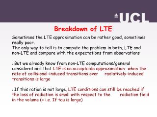
Breakdown of LTE. Sometimes the LTE approximation can be rather good, sometimes really poor. The only way to tell is to compute the problem in both, LTE and non-LTE and compare with the expectations from observations

Breakdown of LTE
E N D
Presentation Transcript
Breakdown of LTE • Sometimes the LTE approximation can be rather good, sometimes really poor. • The only way to tell is to compute the problem in both, LTE and non-LTE and compare with the expectations from observations • But we already know from non-LTE computations/general considerations that LTE is an acceptable approximation when the rate of collisional-induced transitions over radiatively-induced transitions is large • If this ration is not large, LTE conditions can still be reached if the loss of radiation is small with respect to the radiation field in the volume (= i.e. If tau is large)
We must exoect: • LTE is a poor approximation in the outer photospheric layers, where radiation is free to escape into space. The cores of strong lines are formed in these high layers => an LTE approach is inapplicable for them • In O stars, radiation field is so large that it dominates over collisions on a large part of the atmosphere and by a large factor • Similarly, in supergiants the density is very low and collisions are just a few. • => in all these cases, we expect a much better interpretation of the data by using models not restricted to LTE.
Photoelectric observations of Hgamma in Theta Leo, compared to a theoretical profile computed in LTE a) The fit to the wing is good, but the observed line core is deeper than the theoretical one b) this is a common failure on LTE computations Auer and Mihalas (1970), Mihalas (1972) found a much better agreement when using non LTE computations
More generally, a better agreement with non LTE is found in the analysis of Vega and Sirius Paschen continuum, Balmer jump and Balmer lines (exclusive to the core) Schild et al (1971) • Fowler (1974) • Dreiling and Bell (198), Bell and Dreiling (1981, 1982)
Similar situation with other lines. The sodium D lines can be matched well by LTE models except within the cores D lines cores in the Sun studied by Curtis and Jefferies (1967), Athay and Canfield (1969)
Non LTE calculations generally show deeper cores than LTE ones, but still sometimes they do not fit: - discrepancy due to non thermal motions? Solar-D lines observations show their profile varies with time and with position on the solar disk. For other stars the spatial information is lost and we need to deal with average properties. Saturated lines are stronger then predicted => turbolence effect? Many stars show spectral lines braodened by large amounts. Ex lines of delta Cas are broadened by ~130km/s, nearly two order of magnitudesmore than what is expected from thermal broadening => rotational Doppler broadening, effect from macroturbolence
Comparison between LTE and non LTE models: a) continuum formation It is usual to define departures from LTE by using the parameter b_i = N_i/ N*_i * = LTE value
1) B Stars (15000 K < Teff < 30000 K) nLTE effects are negligible for main sequence B stars (log g = 4) Atmospheres are very dense=> collisions force LTE nLTE effects become important for giants and supergiants => here radiative processes dominate over collisional ones The effect on the continuum jumps at the Lyman, Balmer and Paschen edges can be substantial
In particular: 1) the Lymal jump DL is increased by nLTE effects This is because for these stars (B stars) in non LTE the ground state is greatly increased => b_1 >>1 amd hence the flux at Lambda < 912A is reduced. We have J_nu < B_nu => the radiation field is controlling the level population but is not able to ionize substantially because is much less than a BB, so n=1 is overpopulated 2) The Balmer junp is reduced as n=2 level is drained (=> 1) by nLTE effects, so b_2 <1. Moreover, it is also b_3 >1 so the opacity contrast across the edge is reduced 3) the Paschen jump is only slightly affected as both b3, b4 are >1, so the opacity contrast stays more or less the same.
As as result, errors in Teff when Teff is computed from the depth of the Balmer jump are negligible for main sequence B stars, but are of order of 350K for log g=3 and ~500K for log g=2. • The parameter Phi=D_P/D_B provides a sensitive indicator of nLTE • effects: • LTE models predict Phi= 0.16-0.17 independent of g • NLTE models predict Phi much larger, increasing with decreasing g
Fig. 7.22 from Mihalas book: late B-type stars • See the effect of the decrease in the Balmer jump DB in B-type stars • As the Paschen jump is almost unchanged => DP/DB increases • Almost no effect for log g = 4, but substantial effects fro lower g • => stars are less dense and radiative effects become important
Fig. 7.23 from Mihalas book: similar effect for middle B-type stars
2) O Stars (Teff > 30000 K) the situation is reversed! nLTE effects are most pronounced for O stars Now the ground state of H is UNDERPOPULATED (opposite to the B stars. Now Jnu > B_nu => more photoionization so level 1 is drained and flux at lambda < 912 A increases => DL (Lyman jump) decreases changes alter the energy output of O stars i.e. The ionizing flux predicted from these sources, which is important for ionizing HII regions In visible, Balmer jump is increased and shows little variation with gravity at the highest T, discrepancy amounts to errors in Teff ~ 15000K
Fig. 7.24 from Mihalas book: in O stars the situation is reversed Here the ordinate is DB: for a given T, it is INCREASED by nLTE effects Also, it shows little variation with g
Comparison between LTE and non LTE models: b) expectations for lines