Linear Algebra
1.14k likes | 1.89k Views
Linear Algebra. Lecturer: Heru Suhartanto, PhD, heru@cs.ui.ac.id Schedule (at C3113): Monday, 10.00 – 11.40 AM Wednesday, 08.00 – 08.50 AM Marking scheme: 2 exams (mid 25%, final 35 %): reqs = attendance 75% 2 quizes, 20% 4 assignments, 20% Reference:

Linear Algebra
E N D
Presentation Transcript
Linear Algebra • Lecturer: • Heru Suhartanto, PhD, heru@cs.ui.ac.id • Schedule (at C3113): • Monday, 10.00 – 11.40 AM • Wednesday, 08.00 – 08.50 AM • Marking scheme: • 2 exams (mid 25%, final 35 %): reqs = attendance 75% • 2 quizes, 20% • 4 assignments, 20% • Reference: • Horward Anton, Elementary Linear Algebra, 8-th Ed, John Wiley & Sons, Inc, 2000 • More information (will be updated soon) at http://telaga.cs.ui.ac.id/WebKuliah/LinearAlgebra06/ Linear Algebra - Chapter 1 [YR2005]
Why studying Linear Algebra? • It is mostly used in Computer Graphics, animation, cars and aero plane designs, etc. • It is frequently used in economics, and other subjects, • It is frequently used in Scientific Computation and industrial application algorithm and application? • It will be used in any area in the future that you will notice later Linear Algebra - Chapter 1 [YR2005]
Systems of Linear Equation and Matrices CHAPTER 1 FASILKOM UI 05
Introduction ~ Matrices • Information in science and mathematics is often organized into rows and columns to form rectangular arrays. • Tables of numerical data that arise from physical observations • Example: (to solve linear equations) • Solution is obtained by performing appropriate operations on this matrix Linear Algebra - Chapter 1 [YR2005]
1.1 Introduction to Systemsof Linear Equations
Linear Equations • In x y variables (straight line in the xy-plane) where a1, a2, & b are real constants, • In n variables where a1, …, an & b are real constants x1, …, xn = unknowns. • Example 1 Linear Equations • The equations are linear (does not involve any products or roots of variables). Linear Algebra - Chapter 1 [YR2005]
Linear Equations • The equations are not linear. • A solution of is a sequence of n numbers s1, s2, ..., snЭ they satisfy the equation when x1=s1, x2=s2, ..., xn=sn (solution set). • Example 2 Finding a Solution Set • 1 equation and 2 unknown, set one var as the parameter (assign any value) • or • 1 equation and 3 unknown, set 2 vars as parameter Linear Algebra - Chapter 1 [YR2005]
Linear Systems / System of Linear Equations • Is A finite set of linear equations in the vars x1, ..., xn • s1, ..., sn is called a solution if x1=s1, ..., xn=sn is a solution of every equation in the system. • Ex. • x1=1, x2=2, x3=-1 the solution • x1=1, x2=8, x3=1 is not, satisfy only the first eq. • System that has no solution : inconsistent • System that has at least one solution: consistent • Consider: Linear Algebra - Chapter 1 [YR2005]
Linear Systems • (x,y) lies on a line if and only if the numbers x and y satisfy the equation of the line. Solution: points of intersection l1 & l2 • l1 and l2 may be parallel: no intersection, no solution • l1 and l2 may intersect at only one point: one solution • l1 and l2 may coincide: infinite many points of intersection, infinitely many solutions Linear Algebra - Chapter 1 [YR2005]
Linear Systems • In general: Every system of linear equations has either no solutions, exactly one solution, or infinitely many solutions. • An arbitrary system of m linear equations in n unknowns: a11x1 + a12x2 + ... + a1nxn = b1 a21x1 + a22x2 + ... + a2nxn = b2 am1x1 + am2x2 + ... + amnxn = bm • x1, ..., xn = unknowns, a’s and b’s are constants • aij, i indicates the equation in which the coefficient occurs and j indicates which unknown it multiplies Linear Algebra - Chapter 1 [YR2005]
Augmented Matrices • Example: • Remark: when constructing, the unknowns must be written in the same order in each equation and the constants must be on the right. Linear Algebra - Chapter 1 [YR2005]
Augmented Matrices • Basic method of solving system linear equations • Step 1: multiply an equation through by a nonzero constant. • Step 2: interchange two equations. • Step 3: add a multiple of one equation to another. • On the augmented matrix (elementary row operations): • Step 1: multiply a row through by a nonzero constant. • Step 2: interchange two rows. • Step 3: add a multiple of one equation to another. Linear Algebra - Chapter 1 [YR2005]
Elementary Row Operations (Example) • r2= -2r1 + r2 • r3 = -3r1 + r3 Linear Algebra - Chapter 1 [YR2005]
Elementary Row Operations (Example) • r2 = ½ r2 • r3 = -3r2 + r3 • r3 = -2r3 Linear Algebra - Chapter 1 [YR2005]
Elementary Row Operations (Example) • r1 = r1 – r2 • r1 = -11/2 r3 + r1 • r2 = 7/2 r3 + r2 • Solution: Linear Algebra - Chapter 1 [YR2005]
Echelon Forms • Reduced row-echelon form, a matrix must have the following properties: • If a row does not consist entirely of zeros the the first nonzero number in the row is a 1 = leading 1 • If there are any rows that consist entirely of zeros, then they are grouped together at the bottom of the matrix. • In any two successive rows that do not consist entirely of zeros, the leading 1 in the lower row occurs farther to the right than the leading 1 in the higher row. • Each column that contains a leading 1 has zeros everywhere else. Linear Algebra - Chapter 1 [YR2005]
Echelon Forms • A matrix that has the first three properties is said to be in row-echelon form. • Example: • Reduced row-echelon form: • Row-echelon form: Linear Algebra - Chapter 1 [YR2005]
Elimination Methods • Step 1: Locate the leftmost non zero column • Step 2: Interchange r2↔ r1. • Step 3: r1 = ½ r1. • Step 4: r3 = r3 – 2r1. Linear Algebra - Chapter 1 [YR2005]
Elimination Methods • Step 5 : continue do all steps above until the entire matrix is in row-echelon form. • r2 = -½ r2 • r3 = r3 – 5r2 • r3 = 2r3 Linear Algebra - Chapter 1 [YR2005]
Elimination Methods • Step 6 : add suitable multiplies of each row to the rows above to introduce zeros above the leading 1’s. • r2 = 7/2 r3 + r2 • r1 = -6r3 + r1 • r1 = 5r2 + r1 Linear Algebra - Chapter 1 [YR2005]
Elimination Methods • 1-5 steps produce a row-echelon form (Gaussian Elimination). Step 6 is producing a reduced row-echelon (Gauss-Jordan Elimination). • Remark: Every matrix has a unique reduced row-echelon form, no matter how the row operations are varied. Row-echelon form of matrix is not unique: different sequences of row operations can produce different row- echelon forms. Linear Algebra - Chapter 1 [YR2005]
Back-substitution • Bring the augmented matrix into row-echelon form only and then solve the corresponding system of equations by back-substitution. • Example: [Solved by back substitution] Linear Algebra - Chapter 1 [YR2005]
Back-Substitution Step 3. Assign arbitrary values to the free variables [parameters], if any Linear Algebra - Chapter 1 [YR2005]
Homogeneous Linear Systems • A system of linear equations is said to be homogeneous if the constant terms are all zero. • Every homogeneous sytem of linear equations is consistent, since all such systems have x1=0,x2=0,...,xn=0 as a solution [trivial solution]. Other solutions are called nontrivial solutions. Linear Algebra - Chapter 1 [YR2005]
Homogeneous Linear Systems • Example: [Gauss-Jordan Elimination] Linear Algebra - Chapter 1 [YR2005]
Homogeneous Linear Systems The corresponding system of equations is Solving for the leading variables yields The general solution is The trivial solution is obtained when s=t=0 Linear Algebra - Chapter 1 [YR2005]
Homogeneous Linear Systems • Theorem: A homogeneous system of linear equations with more unknowns than equations has infinitely many solutions. Linear Algebra - Chapter 1 [YR2005]
Matrix Notation and Terminology • A matrix is a rectangular array of numbers with rows and columns. • The numbers in the array are called the entries in the matrix. • Examples: • The size of a matrix is described in terms of the number of rows and columns its contains. • A matrix with only one column is called a column matrix or a column vector. • A matrix with only one row is called a row matrix or a row vector. Linear Algebra - Chapter 1 [YR2005]
Matrix Notation and Terminology • aij = (A)ij = the entry in row i and column j of a matrix A. • 1 x n row matrix a = [a1 a2 ... an] • m x 1 column matrix • n x n matrix • A matrix A with n rows and n columns is called a square matrix of order n. Main diagonal of A = {a11, a22, ..., ann} Linear Algebra - Chapter 1 [YR2005]
Operations on Matrices • Definition: • Two matrices are defined to be equal if they have the same size and their corresponding entries are equal. • If A = [aij] and B = [bij] have the same size, then A=B if and only if (A)ij=(B)ij, or equivalently aij=bij for all i and j. • Definition: • If A and B are matrices of the same size, then the sum A+B is the matrix obtained by adding the entries of B to the corresponding entries of A, and the difference A–B is the matrix obtained by subtracting the entries of B from the corresponding entries of A. Matrices of different sizes cannot be added or subtracted. Linear Algebra - Chapter 1 [YR2005]
Operations on Matrices • If A = [aij] and B = [bij] have the same size, then (A+B)ij = (A)ij + (B)ij = aij + bij and (A-B)ij = (A)ij – (B)ij = aij - bij • Definition: • If A is any matrix and c is any scalar, then the product cA is the matrix obtained by multiplying each entry of the matrix A by c. The matrix cA is said to be a scalar multiple of A. • If A = [aij], then (cA)ij = c(A)ij = caij. Linear Algebra - Chapter 1 [YR2005]
Operations on Matrices • Definition If A is an mxr matrix and B is an rxn matrix, then the product AB is the mxn matrix whose entries are determined as follows. To find the entry in row i and column j of AB, single out row i from the matrix A and column j from the matrix B. Multiply the corresponding entries from the row and column together and then add up the resulting products. Linear Algebra - Chapter 1 [YR2005]
Partitioned Matrices • A matrix can be subdivided or partitioned into smaller matrices by inserting horizontal and vertical rules between selected rows and columns. • For example, nexts are three possible partitions of a general 3 x 4 matrix A – • the first is a partition of A into four submatrices A11,A12,A21, and A22. • The second is a partitioned of A into its row matrices r1,r2, and r3. • The third is a partitioned of A into its column matrices c1,c2,c3 and c4. Linear Algebra - Chapter 1 [YR2005]
Partitioned Matrices Linear Algebra - Chapter 1 [YR2005]
Matrix Multiplication by Columns and by Rows • Let A and B be matrices whose product is noted as AB, • J-th column of matrix AB = A [ j-th column matrix of B], • I-th row of AB = [ I-th row of matrix A] B Linear Algebra - Chapter 1 [YR2005]
Matrix Products as Linear Combinations Linear Algebra - Chapter 1 [YR2005]
Matrix Form of a Linear System Linear Algebra - Chapter 1 [YR2005]
Transpose of a Matrix • If A is any m x n matrix then the transpose of A, denoted by AT, is defined to be the n x m matrix that results from interchanging the rows and the columns of A. • For example Linear Algebra - Chapter 1 [YR2005]
Properties of Matrix Operations • ab = ba for real numbers a & b, but AB ≠ BA even if both AB & BA are defined and have the same size. • Example: Linear Algebra - Chapter 1 [YR2005]
Theorem: Properties of A+B = B+A A+(B+C) = (A+B)+C A(BC) = (AB)C A(B+C) = AB+AC (B+C)A = BA+CA A(B-C) = AB-AC (B-C)A = BA-CA a(B+C) = aB+aC a(B-C) = aB-aC Math Arithmetic (Commutative law for addition) (Associative law for addition) (Associative for multiplication) (Left distributive law) (Right distributive law) (a+b)C = aC+bC (a-b)C = aC-bC a(bC) = (ab)C a(BC) = (aB)C Properties of Matrix Operations Linear Algebra - Chapter 1 [YR2005]
Properties of Matrix Operations • Proof (d): • Proof for both have the same size: • Let size A be r x m matrix, B & C be m x n (same size). • This makes A(B+C) an r x n matrix, follows that AB+AC is also an r x n matrix. • Proof that corresponding entries are equal: • Let A=[aij], B=[bij], C=[cij] • Need to show that [A(B+C)]ij = [AB+AC]ij for all values of i and j. • Use the definitions of matrix addition and matrix multiplication. Linear Algebra - Chapter 1 [YR2005]
Properties of Matrix Operations • Remark: In general, given any sum or any product of matrices, pairs of parentheses can be inserted or deleted anywhere within the expression without affecting the end result. Linear Algebra - Chapter 1 [YR2005]
Zero Matrices • A matrix, all of whose entries are zero, such as • A zero matrix will be denoted by 0 or 0mxn for the mxn zero matrix. 0for zero matrix with one column. • Properties of zero matrices: • A + 0 = 0 + A = A • A – A = 0 • 0 – A = -A • A0 = 0; 0A = 0 Linear Algebra - Chapter 1 [YR2005]
Identity Matrices • Square matrices with 1’s on the main diagonal and 0’s off the main diagonal, such as • Notation: In = n x n identity matrix. • If A = m x n matrix, then: • AIn = A and InA = A Linear Algebra - Chapter 1 [YR2005]
Identity Matrices • Example: • Theorem: If R is the reduced row-echelon form of an n x n matrix A, then either R has a row of zeros or R is the identity matrix In. Linear Algebra - Chapter 1 [YR2005]
Identity Matrices • Definition: If A & B is a square matrix and same size Э AB = BA = I, then A is said to be invertible and B is called an inverse of A. If no such matrix B can be found, then A is said to be singular. • Example: Linear Algebra - Chapter 1 [YR2005]
Properties of Inverses • Theorem: • If B and C are both inverses of the matrix A, then B = C. • If A is invertible, then its inverse will be denoted by the symbol A-1. • The matrix is invertible if ad-bc ≠ 0, in which case the inverse is given by the formula Linear Algebra - Chapter 1 [YR2005]