Download
1 / 62
660 likes | 937 Views
Cloud Scheduling. Presented by: Muntasir Raihan Rahman and Anupam Das CS 525 Spring 2011 Advanced Distributed Systems. Papers Presented. Quincy: Fair Scheduling for Distributed Computing Clusters @ SOSP 2009.

E N D
Cloud Scheduling Presented by: Muntasir Raihan Rahman and Anupam Das CS 525 Spring 2011 Advanced Distributed Systems Department of Computer Science, UIUC
Papers Presented Quincy: Fair Scheduling for Distributed Computing Clusters @ SOSP 2009 Michael Isard, VijayanPrabhakaran, Jon Currey, UdiWieder, KunalTalwar, Andrew Goldberg @ MSR Silicon Valley Improving MapReduce Performance in Heterogeneous Environments @ OSDI 2008 MateiZahari, Andy Konwinski, Anthony D. Joseph. Randy Katz, Ion Stoica @ UC Berkeley RAD Lab Reining in the Outliers in Map-Reduce Clusters using Mantri @ OSDI 2010 Ganesh Ananthanarayanan, Ion Stoica @ UC Berkeley RAD Lab, SrikanthKandula, Albert Greenberg @ MSR, Yi Lu @ UIUC, BikashSaha, Edward Harris @ Microsoft Bing Department of Computer Science, UIUC
Quincy: Fair Scheduling for Distributed Computing Clusters [@ SOSP 2009] Michael Isard, VijayanPrabhakaran, Jon Currey, UdiWieder, KunalTalwar, and Andrew Goldberg @ MSR Silicon Valley Some of the slide contents / figures have been taken from the author’s presentation Department of Computer Science, UIUC
Motivation • Fairness: • Existing dryad scheduler unfair [greedy approach]. • Subsequent small jobs waiting for a large job to finish. • Data Locality: • HPC jobs fetch data from a SAN, no need for co-location of data and computation. • Data intensive workloads have storage attached to computers. • Scheduling tasks near data improves performance. Department of Computer Science, UIUC
Fair Sharing • Job X takes t seconds when it runs exclusively on a cluster . • X should take no more than Jt seconds when cluster has J concurrent jobs. • Formally, for N computers and J jobs, each job should get at-least N/J computers. Department of Computer Science, UIUC
Quincy Assumptions • Homogeneous clusters • Heterogeneity is discussed in next paper [LATE scheduler] • Global uniform cost measure • E.g. Quincy assumes that the cost of preempting a running job can be expressed in the same units as the cost of data transfer. Department of Computer Science, UIUC
Fine Grain Resource Sharing • For MPI jobs, coarse grain scheduling • Devote a fixed set of computers for a particular job • Static allocation, rarely change the allocation • For data intensive jobs (map-reduce, dryad) • We need fine grain resource sharing • multiplex all computers in the cluster between all jobs • Large datasets attached to each computer • Independent tasks (less costly to kill a task and restart) Department of Computer Science, UIUC
Example of Coarse Grain Sharing Department of Computer Science, UIUC
Example of Fine Grain Sharing Department of Computer Science, UIUC
Goals of Quincy • Fair sharing with locality. • N computers, J jobs, • Each job gets at-least N/J computers • With data locality • place tasks near data to avoid network bottlenecks • Feels like a multi-constrained optimization problem with trade-offs! • Joint optimization of fairness and data locality • These objectives might be at odds! Department of Computer Science, UIUC
Cluster Architecture Department of Computer Science, UIUC
Baseline: Queue Based Scheduler Department of Computer Science, UIUC
Flow Based Scheduler = Quincy • Main Idea: [Matching = Scheduling] • Construct a graph based on scheduling constraints, and cluster architecture. • Assign costs to each matching. • Finding a min cost flow on the graph is equivalent to finding a feasible schedule. • Each task is either scheduled on a computer or it remains unscheduled. • Fairness constrains number of tasks scheduled for each job. Department of Computer Science, UIUC
New Goal • Minimize matching cost while obeying fairness constraints. • Instead of making local decisions [greedy], solve it globally. • Issues: • How to construct the graph? • How to embed fairness and locality constraints in the graph? • Details in appendix of paper Department of Computer Science, UIUC
Graph Construction • Start with a directed graph representation of the cluster architecture. Department of Computer Science, UIUC
Graph Construction (2) • Add an unscheduled node Uj. • Each worker task has an edge to Uj. • There is a single edge from Uj to the sink. • High cost on edges from tasks to Uj. • The cost and flow on the edge from Uj to the sink controls fairness. • Fairness controlled by adjusting the number of tasks allowed for each job Department of Computer Science, UIUC
Graph Construction (3) • Add edges from tasks (T) to computers (C), racks (R), and the cluster (X). • cost(T-C) << cost(T-R) << cost(T-X). • Control over data locality. • 0 cost edge from root task to computer to avoid preempting root task. Department of Computer Science, UIUC
A Feasible Matching • Cost of T-U edge increases over time • New cost assigned to scheduled T-C edge: increases over time Department of Computer Science, UIUC
Final Graph Department of Computer Science, UIUC
Workloads • Typical Dryad jobs (Sort, Join, PageRank, WordCount, Prime). • Prime used as a worst-case job that hogs the cluster if started first. • 240 computers in cluster. 8 racks, 29-31 computers per rack. • More than one metric used for evaluation. Department of Computer Science, UIUC
Experiments Department of Computer Science, UIUC
Experiments (2) Department of Computer Science, UIUC
Experiments (3) Department of Computer Science, UIUC
Experiments (4) Department of Computer Science, UIUC
Experiments (5) Department of Computer Science, UIUC
Conclusion • New computational model for data intensive computing. • Elegant mapping of scheduling to min cost flow/matching. Department of Computer Science, UIUC
Discussion Points • Min cost flow recomputed from scratch each time a change occurs • Improvement: incremental flow computation. • No theoretical stability guarantee. • Fairness measure: control number of tasks for each job, are there other measures? • Correlation constraints? • Other models: auctions to allocate resources. • Selfish behavior: jobs manipulating costs. • Heterogeneous data centers. • Centralized Quincy controller: single point of failure. Department of Computer Science, UIUC
Improving MapReduce Performance in Heterogeneous Environments MateiZahari, Andy Konwinski, Anthony D. Joseph. Randy Katz, Ion Stoica Some of the slide contents have been taken from the original presentation Department of Computer Science, UIUC
k1 v1 k1 v1 k2 v2 k1 v3 k1 v3 k1 v5 k2 v2 k2 v4 k2 v4 k1 v5 Background Map-Reduce Phases Input records Output records map reduce Split reduce map Split shuffle Department of Computer Science, UIUC
Motivation • MapReduce is becoming popular • Open-source implementation: Hadoop, used by Yahoo!, Facebook, • Scale: 20 PB/day at Google, O(10,000) nodes at Yahoo, 3000 jobs/day at Facebook • Utility computing services like Amazon Elastic Compute Cloud (EC2) provide cheap on-demand computing • Price: 10 cents / VM / hour • Scale: thousands of VMs • Caveat: less control over performance • So the smallest increase in performance has significant impact Department of Computer Science, UIUC
Motivation Performance depends MapReduce (Hadoop) Task Scheduler (handles stragglers) The task scheduler makes its decision based on the assumption that cluster nodes are homogeneous. However, this assumption does not hold in heterogeneous environments like Amazon EC2. Department of Computer Science, UIUC
Goal Improve the performance of speculative executions. Speculative execution deals with rerunning stragglers. • Define a new scheduling metric. • Choosing the right machines to run speculative tasks. • Capping the amount of speculative executions. Department of Computer Science, UIUC
Speculative Execution Slow nodes/stragglers are the main bottleneck for jobs not finishing in time. So, to reduce response time stragglers are speculatively executed on other free nodes. Node 1 Node 2 How can this be done in a heterogeneous environment? Department of Computer Science, UIUC
Speculative Execution in Hadoop Associated Progress score Task ϵ[0,1] Progress Score Map Task Fraction of data read 1/3*Copy Phase + 1/3*Sort Phase + 1/3*Reduce Phase Progress depends Reduce Task E.g. a task halfway through reduce phase scores=1/3*1+1/3*1+1/3*1/2=5/6 Speculative execution threshold : progress < avgProgress – 0.2 Department of Computer Science, UIUC
Hadoop’s Assumption Nodes can perform work at exactly the same rate Tasks progress at a constant rate throughout time There is no cost to launching a speculative task on an idle node The three phases of execution take approximately same time Tasks with a low progress score are stragglers Maps and Reduces require roughly the same amount of work Department of Computer Science, UIUC
Breaking Down the Assumptions • The first 2 assumptions talk about homogeneity. But heterogeneity exists due to- • Multiple generations of Hardware. • Co-location of multiple VMs on the same physical host. Department of Computer Science, UIUC
Breaking Down the Assumptions Assumption 3:There is no cost to launching a speculative task on an idle node Not true in situations where resources are shared. E.g. Network Bandwidth Disk I/O operation Department of Computer Science, UIUC
Breaking Down the Assumptions Assumption 4: The three phases of execution take approximately the same time. The copy phase of the reduce task is the slowest while the other 2 phases are relatively faster. Suppose 40% of the reducers have finished the copy phase and quickly completed their remaining task. The Remaining 60% are near the end of copy phase. Avg progress: 0.4*1+0.6*1/3=60% Progress of the 60% reduce tasks= 33.33% progress < avgProgress – 0.2 Department of Computer Science, UIUC
Breaking Down the Assumptions Assumption 5: Tasks with a low progress score are stragglers. Suppose a task has finished 80% of its work, and from that point onward gets really slow. But due to the 20% threshold it can never be speculated. 80% < 100%-20% Department of Computer Science, UIUC
Problems With Speculative Execution • Too manybackups, thrashing shared resources like network bandwidth • Wrong tasks backed up • Backups may be placed on slow nodes • Example: Observed that ~80% of reduces backed up, most of them lost to originals; network thrashed Department of Computer Science, UIUC
Idea: Use Progress Rate Instead of using progress score, compute progress rates, and backup tasks that are “far enough” below the mean Problem: can still select the wrong tasks Progress Score Progress Rate = Execution Time Department of Computer Science, UIUC
Progress Rate Example A job with 3 tasks 1 min 2 min Node 1 1 task/min Node 2 3x slower 1.9x slower Node 3 Time (min) Department of Computer Science, UIUC
Progress Rate Example What if the job had 5 tasks? 2 min Free Slot Task1 Task4 Node 1 Progress rate Node2=0.33 Node3=0.53 Node2 selected Node 2 Task2 time left: 1 min Node 3 Task3 Task5 time left: 1.8 min Task5 Time (min) Node 2 is slowest, but should back up Node 3’s task! Department of Computer Science, UIUC
LATE Scheduler • Longest Approximate Time to End • Primary assumption: best task to execute is the one that finishes furthest into the future • Secondary: tasks make progress at approx. constant rate.Caveat-can still select the wrong tasks 1- Progress Score Estimated time left= Progress Rate Department of Computer Science, UIUC
LATE Scheduler 2 min Task 1 Task 4 Node 1 Copy of Task 5 Estimated time left: (1-0.66) / (1/3) = 1 min Node 2 Task 2 Progress = 66% Estimated time left: (1-0.05) / (1/1.9) = 1.8 min Node 3 Task3 Task 5 Progress = 5.3% Time (min) LATE correctly picks Node 3 Department of Computer Science, UIUC
Other Details of LATE • Cap the number of speculative tasks • SpeculativeCap-10% • Avoid unnecessary speculations • Limit contention and hurting throughput • Select fast node to launch backups • SlowNodeThreshold–25th percentile • Based on total work performed • Only back-up tasks that are sufficiently slow • SlowTaskThreshold–25th percentile • Based on task progress rate • Does not consider data locality Department of Computer Science, UIUC
Evaluation Environment • Environments: • Amazon EC2 (200-250 nodes) • Small Local Testbed (9 nodes) • Heterogeneity Setup: • Assigning a varying number of VMs to each node • Running CPU and I/O intensive jobs to intentionally create stragglers Department of Computer Science, UIUC
EC2 Sort with Heterogeneity Each host sorted 128MB with a total of 30GB data Average 27% speedup over native, 31% over no backups Department of Computer Science, UIUC
EC2 Sort with Stragglers Each node sorted 256MB with a total of 25GB of data Stragglers created with 4 CPU (800KB array sort) and 4 disk (dd tasks) intensive processes Average 58% speedup over native, 220% over no backups Department of Computer Science, UIUC
EC2 Grep and Wordcount with Stragglers Grep WordCount • 36% gain over native • 57% gain over no backups • 8.5% gain over native • 179% gain over no backups Department of Computer Science, UIUC