Download
1 / 1
10 likes | 122 Views
Introduction

E N D
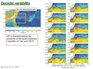
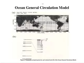
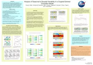
Introduction The Global Modeling and Assimilation Office (GMAO) coupled general circulation model (CGCMv1) is used primarily for seasonal forecasts, but several long (100-year) simulations have also been completed with this model. In this study, we examine the internal variability of the coupled atmosphere-land-ocean system and compare it with observations. The focus is on the ability of the coupled system to reproduce the leading modes of sea surface temperature (SST) and atmospheric variability on time scales ranging from seasonal to decadal. The analysis includes an assessment of how the variability is impacted by changes in horizontal resolution. Decadal Variability In Figure 4, the model shows some variability in the strength and timing of the ENSO events on decadal or sub-decadal time scales. Both models also show a realistic North Pacific Index (NPI, Figure 7), which quantifies changes in strength of the Aleutian Low during northern winter. There is evidence of decadal variability in the SSTs in the NPI region, but the link to the tropical SST patterns is weak (Figure 8). Model Description Atmosphere: NSIPP-1 AGCM (Bacmeister et al. 2000) 4th order global grid point dynamical core (Suarez and Takacs 1995) RAS convection scheme (Moorthi and Suarez 1992) Resolution: 2° latitude by 2.5° longitude by 34 sigma levels Ocean: Poseidon v4 quasi-isopycnal reduced gravity OGCM (Schopf and Loughe 1995) Thermodynamic ice model Bulk mixed layer for Arctic Ocean Deep layer temperature and salinity interpolated from 1994 World Ocean Atlas (Levitus et al. 1994). Resolution: 1/3° latitude by 5/8° longitude by 27 layers Land: Mosaic v3 (Koster and Suarez 1992, 1996) The models are coupled once per day, and no flux corrections are employed. A second experiment with this model is shown; this experiment employs higher horizontal resolution in the atmosphere (1° latitude by 1.25° longitude). Some results are presented from an AMIP run, where the atmospheric component is run with prescribed SSTs from observations. First EOF and PC of SST ENSO Signal The CGCMv1 internal variability includes ENSO warm and cold events in the tropical Pacific (Figure 4a); however, the amplitude and periodicity of these events are problematic. The events are too weak in amplitude, with the maximum anomaly rarely above 2.5°C. Only the strongest events reach the west coast of South America. Also, the return period of the ENSO events is too biennial. The CGCMv1 with higher resolution shows several improvements (Figure 4b). First, this run is capable of producing stronger ENSO events. Most of the strong and weak ENSO events in this run reach the west coast of South America. The events also seem to persist for a longer period, and the signal is not as biennial as the lower resolution version. There are still some limitations to the ENSO events that are not mitigated by the change in resolution. The ENSO signal is too narrow when compared to observations (Figure 5). Very little of correlation signal can be found off the equator in the Pacific or even in other tropical oceans. The corresponding time series associated with the ENSO EOF pattern again shows the biennial nature of the ENSO signal in the model. Power spectra of the principal components show that the predominant period in the CGCMv1 is close to 2 years (Figure 5d). The higher resolution version of the model has a broader peak of 2.5 to 3.5 years; however, nature has peaks at 4-7 years. B A D C Figure 5. First Empirical Orthogonal Function and corresponding Principal Component for sea surface temperature. Results from CGCMv1 (A), higher resolution model run (B), and SST from observations (C). Power spectra of the PC time series (D), where black is observations, red is CGCMv1, and blue is the higher resolution model run. Annual Mean and Seasonal Climatology There are several differences in annual mean sea surface temperature (SST) between the two model runs (Figure 1). The SST over several regions is over 0.5°C cooler in the higher resolution run, although a few areas in the Pacific do show warmer SST. The eastern Equatorial Pacific shows improvement with increased resolution, especially in the SSTs east of 90°W (Figure 2). Both runs show an improved realization of zonal wind stress over the AMIP run. The seasonal cycle of SST and wind stress in the Equatorial Pacific is affected by the change in resolution (Figure 3). The phasing of the zonal wind stress cycle is better in the higher resolution run, although the amplitude of the anomaly is much weaker. This wind stress pattern and reduced bias leads to a better phasing of the seasonal cycle of SST east of 90°W and more realistic propagation of during the warm season. However, the amplitude of the SST seasonal cycle is still too weak. ENSO Response The upper atmospheric response to ENSO events is presented in Figure 6. The pattern of the response of the coupled model is good, although the response in the subtropics is somewhat weak. The higher resolution version of the model has a stronger response in the mid-latitudes and over the tropics, specifically over the Indian Ocean. North Pacific Index Interannual Anomaly of Equatorial Pacific SST for CGCMv1 Correlation of NINO3 and 200mb Heights A A Figure 8. Empirical Orthogonal Function and associated Principal Component of SST for CGCMv1 (left) and the higher resolution run (right). The fourth (left) and second (right) EOFs show the pattern usually associated with the Pacific Decadal Oscillation (PDO). Annual Mean Sea Surface Temperature Equatorial Pacific Annual Mean Summary The GMAO CGCMv1 reproduces several climate signals on the seasonal to decadal time scales, although some aspects of these events are still not well-represented. Increased horizontal resolution tends to improve the realism of the variability. Higher atmospheric resolution has less bias in the eastern Equatorial Pacific, which corresponds to better representations of the seasonal cycle and ENSO events in this area. This model is used to generate the seasonal forecasts at the GMAO. Future work to analyze the behavior of the model in the seasonal-to-interannual time scale may help diagnose anomalous results in the forecasts. Figure 7. North Pacific Index of normalized sea level pressure anomalies. The black line represents the raw index from CGCMv1. The red line is a running mean of the raw index, and the blue line is the running mean of the observed index (adapted from Trenberth and Hurrell, 1994). The North Pacific Index is the weighted average of extended winter SLP anomalies over the region from 30°N to 65°N and from 160°E to 140°W. B Figure 1. Annual mean SST bias from Reynolds and Smith (1994) SST (top). Difference in annual mean SST between the higher and lower resolution runs (bottom). The contour interval on the top plot is 1°C and on the bottom plot is 0.5°C. Figure 2. Annual mean sea surface temperature (top) and zonal wind stress (bottom) across the Pacific Ocean averaged from 2°S to 2°N. B References Bacmeister, J., P. Pegion, S. Schubert, and M.Suarez, 2000: Atlas of seasonal means simulated by the NSIPP 1 Atmospheric GCM, NASA Tech. Memo. 104606, Vol. 17. Koster, R. and M. Suarez, 1992: Modeling the land surface boundary in climate models as a composite of independent vegetation stands. J. Geophys. Res., 97, 2697-2715. Koster, R. and M. Suarez, 1996: Energy and water balance calculations in the Mosaic LSM, NASA Tech. Memo. 104606, Vol. 9. Levitus, S., R. Burgett, T. Boyer, 1994:World Ocean Atlas 1994, Vol. 3: Salinity. NOAA Atlas NESDIS 3,U.S. Gov. Printing Office, Wash., D.C.,99 pp. Moorthi, S. and M. Suarez, 1992: Relaxed Arakawa-Schubert: a parameterization of moist convection for general circulation models. Mon. Weather Rev., 120, 978-1002. Rayner, N. A., D. E. Parker, E. B. Horton, C. K. Folland, L. V. Alexander, D. P. Rowell, E. C. Kent, and A. Kaplan, 2003: Global analyses of sea surface temperature, sea ice, and night marine air temperature since the late nineteenth century. J. Geophys. Res., 99, 20323-20344. Reynolds, W. and T. Smith, 1994: Improved global sea surface temperature analyses using optimum interpolation. J. Climate, 7, 929-948. Schopf, P. S., and A. Loughe, 1995: A reduced-gravity isopycnal model:Hindcast of El Nino. Mon. Wea. Rev., 123, 926-941. Suarez, M. and L. Takacs, 1996: Dynamical aspects of climate simulations using the GEOS GCM, NASA Tech. Memo. 104606, Vol 5. Trenberth, K. E., and J. W. Hurrell, 1994: Decadal atmospheric-ocean variations in the Pacific. Climate Dyn., 9, 303-319. Vintzileos, A., M. M. Rienecker, M. J. Suarez, S. K. Miller, P. J. Pegion, and J. T. Bacmeister, 2003: Simulation of the El Nino-Southern Oscillation phenomenon with NASA’s Seasonal-to-Interannual Prediction Project coupled general circulation model. CLIVAR Exchanges, 8(4), 25-27. Seasonal Cycle of SST and Wind Stress in the Equatorial Pacific Ocean C Figure 4. Hovmüller diagrams of interannual anomaly of sea surface temperature for CGCMv1 (A) and CGCMv1 with higher horizontal resolution (B). Plots show 87 years of each run, starting from the lower left panel. Figure 3. Seasonal anomaly of sea surface temperature (top row) and zonal wind stress (bottom row). Far left: Observations, center left: results from an atmosphere-land run with prescribed SSTs, center right: model results from lower resolution experiment, far right: model results for higher resolution experiment. Figure 6. Pointwise correlation of northern winter NINO3 sea surface temperature index and 200 mb heights for observations (A), CGCMv1 (B), and CGCMv1 with higher resolution (C). The NINO3 index is an area-weighted average of SST over the region defined from 5°S to 5°N and 150°W to 90°W. Analysis of Seasonal to Decadal Variability in a Coupled General Circulation Model Sonya K. Miller1, Michele M. Rienecker2, Max J. Suarez2, Siegfried D. Schubert2, Philip J. Pegion1, Julio T. Bacmeister3 Affiliations: Global Modeling and Assimilation Office, NASA/GSFC (1) Science Applications International Corporation (2) NASA/Goddard Space Flight Center (3) Goddard Earth Sciences and Technology Center, UMBC Greenbelt, MD Contact Information: Sonya.K.Miller.1@gsfc.nasa.gov http://gmao.gsfc.nasa.gov