Download
1 / 62
620 likes | 736 Views
Lecture VIII: Time And Global Clocks. CMPT 401 Summer 2007 Dr. Alexandra Fedorova. A Distributed Computation With Data Dependencies. System A. System B. A waits for B. B waits for C. System C. Ask data from System C Respond to System A. Ask work from System B Compute

E N D
Lecture VIII: Time And Global Clocks CMPT 401 Summer 2007 Dr. Alexandra Fedorova
A Distributed Computation With Data Dependencies System A System B A waits for B B waits for C System C • Ask data from System C • Respond to System A • Ask work from System B • Compute • Send result to user System C became unresponsive
Detecting and Fixing the Problem • User gets no response from System A • How do we detect that System C is causing the problem? • Easy too detect if we get a snapshot of a global state • Constructing global state in an asynchronous distributed system is a difficult problem
A Naïve Approach • Each system records each event it performed and its timestamp • Suppose events in the this system happened in this real order: • Time Tc0: System C sent data to System B (before it stopped responding) • Time Ta0: System A asked for work from System B • Time Tb0: System B asked for data from System C Tc0 Ta0 Tb0
A Naïve Approach (cont) • Ideally, we will construct real order of events from local timestamps and detect this dependency chain: System A Ta System A asked for work Tb System B System B asked for data System C sent data System C Tc
A Naïve Approach (cont) • But in reality, we do not know if Tc occurred before Ta and Tb, because in an asynchronous distributed system clocks are not synchronized! System A Ta System A asked for work Tb System B System B asked for data System C sent data System C sent data System C Tc Tc
This Lecture’s Topic • We will learn how to solve this problem in an asynchronous distributed system • Our goal is to construct a consistent global state in presence of unsynchronized local clocks • We will begin by creating a formal model for • Distributed computation • Event precedence in a distributed computation • We will use event precedence model to define consistent global state • Then we will learn to construct consistent global states
Model of a Distributed Computation • Collection of processes p0, …, pn • Processes communicate by sending messages • Event send(m)enqueues message m on the sending end • Event receive(m)dequeues message m on the receiving end • Events ei0, ei1, … , einare steps of distributed computation at processpi • hi = ei0, ei1, … , einis a local history of pi
Events and Causal Precedence • In an asynchronous distributed system there is no notion of global clock • Events cannot be ordered according to some real order • We can only talk about causal event ordering, that is if one event affects the outcome of another event • For example events send(m) and receive(m) are in causal order, because receive(m)could not have occurred before send(m)
Formal Rules for Ordering of Events • If local events precede one another, then they also precede one another in the global ordering: • If eik ,eimЄ hi and k < m, then eik→eim • Sending a message always precedes receipt of that message: • If ei= send(m) and ej= receive(m), then ei→ej • Event ordering is associative: • If e → e’ and e’ → e”, then e → e”
Space-time Diagram of a Distributed Computation e11 e12 e13 e14 e15 e22 e21 e16 e31 e32 e33 e34 e35 e36 e23 p1 p2 p3 e21→e36 e22 || e36
Cuts of a Distributed Computation • Suppose there is an external monitor process • External monitor constructs a global state: • Asks processes to send it local history • Global state constructed from these local histories is a cut of a distributed computation
Example Cuts e21 e11 e12 e13 e14 e16 e31 e15 e23 e32 e33 e34 e35 e36 e22 p1 p2 p3 C’ C
Consistent vs. Inconsistent Cuts • A cut is consistent if for any event e included in the cut, any event e’ that causally precedes e is also included in that cut • For cut C: (e Є C) Λ (e’→ e) => e’ Є C
Are These Cuts Consistent? e21 e11 e12 e13 e14 e16 e31 e15 e23 e32 e33 e34 e35 e36 e22 p1 p2 p3 Events in the frontier of the cut C
Are These Cuts Consistent? causally precedes e36 e22 e11 e12 e13 e14 e15 e21 e16 e23 e32 e33 e34 e35 e36 e31 …but not included in C inconsistent included in C C’
Cuts and Global State • Recall that our goal is to construct a consistent global state • We’d like to get a snapshot of a distributed system as would have been observed by a perfect observer • A consistent cut corresponds to a consistent global state • What’s next: we will learn how to construct consistent cuts in the absence of synchronized clocks • Consistent global states can be constructed via: • Active monitoring • Passive monitoring
Passive vs. Active Monitoring • Passive monitoring: • There is a process p0external to the distributed computation • There are processes pi (1 ≤ i ≤ n), part of the computation • Each process pi sends to p0a timestamp of each event it executes • Active monitoring: • There is a process p0 external to the distributed computation • When p0 desires to find out the state of the system it asks all processes pi to send its state
Passive vs. Active Monitoring • You need both passive and active monitoring • The kind of monitoring you use depends on what property of a distributed system you are trying to detect • Passive monitoring gives you more information about the distributed computation than active monitoring • Passive monitoring records the entire event history • Passive monitoring useslogical clocks or vector clocks – a way to timestamp an event in the absence of global clock • Active monitoring does not depend of special clocks, but it is also less powerful
What Do We Need to Know to Construct a Consistent Cut? causally precedes e36 e22 e11 e12 e13 e14 e15 e21 e16 e23 e32 e33 e34 e35 e36 e31 We must know the causal ordering of events. If we do we can detect an inconsistent cut …but not included in C inconsistent included in C C’
Constructing a Consistent Cut Via Passive Monitoring • We must know the causal ordering of event • If there was a global clock, we would detect this as follows: • RC(e) – timestamp of event e given by a global clock • Clock condition: e’→ e => RC(e) < RC(e’) • What to do if there is no global clock? • We will use logical clocks and vector clocks
Logical Clocks • Each process maintains a local value of a logical clock LC • Logical clock of process p counts how many events in a distributed computation causally preceded the current event at p (including the current event). • LC(ei) – the logical clock value at process piat event ei • Suppose we had a distributed system with only a single process e11 e12 e13 e14 e15 e16 LC=1 LC=2 LC=3 LC=4 LC=5 LC=6
Logical Clocks (cont.) • In a system with more than one process logical clocks are updated as follows: • Each message m that is sent contains a timestamp TS(m) • TS(m) is the logical clock value associated with sending event at the sending process e11 e12 e13 e14 e15 e16 LC=1 send(m) TS(m) = 1
Logical Clocks (cont) • When the receiving process receives message m, it updates its logical clock to: max{LC, TS(m)} + 1 e11 e12 e13 e14 e15 e16 e22 e21 LC=1 send(m) TS(m) = 1 What is the LC value of e22? LC=1 LC=2
Illustration of a Logical Clock 1 2 \ 3 4 5 6 7 p1 1 5 6 p1 1 2 3 4 5 7 p1
Causal Delivery with Logical Clocks • We have a external monitor process p0 • Each process pi sends an event notification message m to p0 after each event ei • To let p0 construct a correct causal ordering of events, we define the following delivery rule for event notification messages: Causal delivery rule: Event notification messages are delivered to p0 in the increasing logical clock timestamp order
Causal Delivery Rule 1 2 3 4 p0 m(LC=1) m(LC=2) m(LC=4) m(LC=3) 1 2 4 5 6 7 p1 1 2 3 4 5 7 p2
Mind the Gap, Please! Oops! 1 2 3 4 p0 m(LC=1) m(LC=2) m(LC=4) m(LC=1) m(LC=3) 1 2 4 5 6 7 p1 1 2 3 4 5 7 p2
Rules to Achieve Causal Delivery • Rule #1: Do not deliver event notification message from a process piunless all messages with smaller timestamps have been delivered • Rule #2: Do not deliver event notification message with a timestamp TS(m) unless received messages with timestamps equal or greater than TS(m) from all other processes
Causal Delivery Rules 1 1 2 p0 m(LC=1) m(LC=2) m(LC=4) m(LC=1) m(LC=3) 1 2 4 5 6 7 p1 1 2 3 4 5 7 p2
Causal Precedence Relation • Using just timestamps from logical clocks does not help us detect whether two events are causally related or concurrent
Causal Precedence or Concurrency? 1 1 2 2 p0 1 2 p1 e11 e11and e22are concurrent e22 1 2 p2
Causal Precedence or Concurrency? 1 1 2 2 p0 1 2 p1 e11 Now e11and e22are causally related But timestamps have not changed!!! e22 1 2 p2
Causal Precedence Relation • Using just timestamps from logical clocks does not help us detect whether two events are causally related or concurrent • A naïve approach: include a local history in the event notification message • Not a good idea: messages will become large • A better idea: vector clocks
Introduction to Vector Clocks • The clock of each process is represented by a vector • The vector dimension is the number of processes in the system • Each entry of a vector clock corresponds to a process • Suppose there are three processes: p1, p2, andp3 • Then the vector clock at each process will look like this: VC[1] – entry for process p1 VC[2] – entry for process p2 VC[3] – entry for process p3
Using Vector Clocks VC[1] = 0 VC[2] = 0 VC[1] = 1 VC[2] = 0 1 p1 Arrives with the message Increment local component to “1” for an internal of “send” event Increment other processes’ components to be no less than at the incoming VC VC[1] = 1 VC[2] = 0 Initialize to 0 1 2 p2 VC[1] = 0 VC[2] = 1 VC[1] = 1 VC[2] = 2 VC[1] = 0 VC[2] = 0 Increment the local component
The Meaning of Vector Clocks • An entry of a vector clock for process pi is the number of events at pi VC[1] = 3 – event count at p1 VC[2] = 0 – event count at p2 VC[3] = 1 – event count at p3 • p1knows for sure how many events it executed • But how can it be sure about p2 and p3? It can’t! • So entries for p2 and p3is what p1thinks about p2 and p3
Meaning of Vector Clocks (cont) • p1 thinks incorrectly about other processes if p1 does not communicate with other processes • Once p1 exchanges messages with other processes, it updates its “thinking” using vector clock timestamps received from other processes
Another Vector Clock Example VC[1] = 1 VC[2] = 0 VC[3] = 0 VC[1] = 3 VC[1] = 2 VC[1] = 4 VC[2] = 1 VC[3] = 3 VC[1] = 6 VC[2] = 1 VC[3] = 3 VC[1] = 5 VC[2] = 1 VC[3] = 3 VC[2] = 1 VC[2] = 1 VC[3] = 3 VC[3] = 0 p1 VC[1] = 0 VC[2] = 1 VC[3] = 0 p2 VC[1] = 1 VC[2] = 2 VC[3] = 4 VC[1] = 4 VC[2] = 3 VC[3] = 4 p3 VC[1] = 5 VC[2] = 1 VC[3] = 6 VC[1] = 0 VC[2] = 0 VC[3] = 1 VC[1] = 1 VC[2] = 0 VC[3] = 4 VC[1] = 1 VC[2] = 0 VC[3] = 5 VC[1] = 1 VC[1] = 1 VC[2] = 0 VC[3] = 3 VC[2] = 0 VC[3] = 2
Causal Precedence or Concurrency? VC[1] = 0 VC[2] = 2 VC[1] = 1 VC[2] = 0 VC[1] = 0 VC[2] = 1 VC[1] = 2 VC[2] = 0 p0 VC[1] = 1 VC[2] = 0 VC[1] = 2 VC[2] = 0 1 2 p1 e11 VC[1] = 0 VC[2] = 2 VC[1] = 0 VC[2] = 1 e11and e22are concurrent e22 1 2 p2
Causal Precedence or Concurrency? VC[1] = 1 VC[2] = 2 VC[1] = 1 VC[2] = 0 VC[1] = 0 VC[2] = 1 VC[1] = 2 VC[2] = 0 p0 Now e11and e22are causally related VC[1] = 1 VC[2] = 0 VC[1] = 2 VC[2] = 0 1 2 p1 e11 VC[1] = 0 VC[2] = 1 VC[1] = 1 VC[2] = 2 e22 1 2 p2
Vector Clocks Detect Causal Precedence • Let us look at timestamps received by observer p0: • In case when events were concurrent: • From p1: • From p2: • In case when events where causally related: • From p1: • From p2: VC[1] = 2 VC[2] = 0 VC[1] = 0 VC[2] = 2 VC[1] = 2 VC[2] = 0 Now the timestamps help detect causal precedence VC[1] = 1 VC[2] = 2
Use Vector Clocks to Construct Consistent Cuts • A consistent cut is a cut that does not include pairwise inconsistent events • So the first step is to understand pairwise inconsistency
Informal Definition of Pairwise Inconsistency • Look at vector timestamps of two events: ei at pi and ej at pj • If at event : ei process pi thinks that process pj executed more events than process pj thinks it has executed at event ej, the events are pairwise inconsistent Example: timestamp at p3 timestamp at p1 • The events are pairwise inconsistent • Process p1 must know better about what it’s doing than process p3 could ever know. VC[1] = 5 VC[2] = 1 VC[3] = 6 VC[1] = 4 VC[2] = 1 VC[3] = 3 p3thinks that p1 has executed 5 events p1has executed 4 events!
Formal Definition of Pairwise Inconsistency • Two events ei and ej ,are pairwise inconsistent if: (VC(ei )[i] < VC(ej)[i]) ٧ (VC(ej )[j] < VC(ei)[j]) the number of events pithinks to have executed at event ei the number of events pjthinks that pj has executed at event ej
Cut Consistency • Among all events in the frontier of the cut, choose each pair of events for pairwise inconsistency • If at least two events are pairwise inconsistent, then the cut is inconsistent
Is this Cut Consistent? VC[1] = 1 VC[2] = 0 VC[3] = 0 VC[1] = 3 VC[1] = 2 VC[1] = 4 VC[2] = 1 VC[3] = 3 VC[1] = 6 VC[2] = 1 VC[3] = 3 VC[1] = 5 VC[2] = 1 VC[3] = 3 VC[2] = 1 VC[2] = 1 VC[3] = 3 VC[3] = 0 p1 VC[1] = 0 VC[2] = 1 VC[3] = 0 p2 VC[1] = 1 VC[2] = 2 VC[3] = 4 VC[1] = 4 VC[2] = 3 VC[3] = 4 p3 VC[1] = 5 VC[2] = 1 VC[3] = 6 VC[1] = 0 VC[2] = 0 VC[3] = 1 VC[1] = 1 VC[2] = 0 VC[3] = 4 VC[1] = 1 VC[2] = 0 VC[3] = 5 VC[1] = 1 VC[1] = 1 VC[2] = 0 VC[3] = 3 VC[2] = 0 VC[3] = 2
And What About This One? VC[1] = 1 VC[2] = 0 VC[3] = 0 VC[1] = 3 VC[1] = 2 VC[1] = 4 VC[2] = 1 VC[3] = 3 VC[1] = 6 VC[2] = 1 VC[3] = 3 VC[1] = 5 VC[2] = 1 VC[3] = 3 VC[2] = 1 VC[2] = 1 VC[3] = 3 VC[3] = 0 p1 VC[1] = 0 VC[2] = 1 VC[3] = 0 p2 VC[1] = 1 VC[2] = 2 VC[3] = 4 VC[1] = 4 VC[2] = 3 VC[3] = 4 p3 VC[1] = 5 VC[2] = 1 VC[3] = 6 VC[1] = 0 VC[2] = 0 VC[3] = 1 VC[1] = 1 VC[2] = 0 VC[3] = 4 VC[1] = 1 VC[2] = 0 VC[3] = 5 VC[1] = 1 VC[1] = 1 VC[2] = 0 VC[3] = 3 VC[2] = 0 VC[3] = 2
Active Monitoring • Recall: we used vector clocks so we can construct consistent global states (or cuts) from processes’ local histories via passive monitoring • Remember, there is another type of monitoring – active monitoring: • Does not depend of vector clocks, but it is less powerful • Active monitoring is also referred to as constructing a distributed snapshot
Distributed Snapshot Protocol (Chandy and Lamport) • Monitor p0 sends “take snapshot” message to all processes pi • If pi receives such “take snapshot” message for the first time, it: • Records its state • Stops doing any activity related to the distributed computation • Relays the “take snapshot” message on all of its outgoing channels • Starts recording a state of its incoming channels – records all messages that have been delivered after the receipt of the first “take snapshot” message