Download
1 / 46
520 likes | 920 Views
Radiometric Correction and Image Enhancement. Radiometric correction Noise removal Atmospheric correction Seasonal compensation Image Reduction and Magnification Image Enhancement Radiometric Enhancement - Contrast stretching

E N D
Radiometric Correction and Image Enhancement • Radiometric correction Noise removal Atmospheric correction Seasonal compensation • Image Reduction and Magnification • Image Enhancement Radiometric Enhancement - Contrast stretching Spatial Enhancement - Filtering - Edge enhancement
Radiometric Correction The repair or adjustment of pixel intensity (DN) values. • Three Types • Noise Removal • Atmospheric Corrections • Seasonal Compensation
Noise Removal Noise is the result of sensor malfunction during the recording or transmittal of data and manifests itself as inaccurate gray level readings or missing data. Line Drop occurs when a sensor either fails to function, like a camera flash on your retina. The result is a line, or partial line, with higher DN values. Fixed with a masked averaging, or low pass, filter (see below). Striping occurs when a sensor goes out of adjustment (improper calibration). The result is a striping pattern in which every nth line contains erroneous data. The problem can be fixed with “de-striping algorithms”.
Line Drop Before Repair After Repair
Atmospheric Correction Correct for atmospheric scattering and absorption effects and restore digital numbers to ground reflectance values
Seasonal Compensation • The compensation for differences in sun elevation. • In temporal studies with images acquired at different times of the year it is important to make an adjustment for differences in brightness associated with sun elevation. This adjustment is made by dividing each image pixel by the sine of the solar elevation for that scene: • New DN = DN of pixel XY / sine(sun elevation). Winter Summer
Image Reduction Also called pyramidal structure for fast display of image
Integer Image Reduction Atlanta Downtown Area
Image Magnification (Or Image expansion)
Image Magnification Atlanta Downtown
Contrast Stretching Most satellite sensors are designed to accommodate a wide range of illumination conditions, from dark boreal forest to highly reflective desert regions. Pixel values in most scenes occupy a small range of values. This results in low display contrast. A contrast enhancement expands the range of “displayed” pixel values and increases image contrast.
Linear Contrast Stretch Grey level values are expanded uniformly to the full range of an eight bit display device. (0-255).
Histogram Equalization Stretch Grey level values are assigned to display levels on the basis of their frequency of occurrence.
Common Symmetric and Skewed Distributions in Remotely Sensed Data
Min-Max Contrast Stretch +1 Standard Deviation Contrast Stretch
Contrast Stretch of Charleston, SC Landsat Thematic Mapper Band 4 Data Original Minimum-maximum +1 standard deviation
Grey Level Thresholding Feature extraction based on a range (min,max) of gray level values. Either the visual inspection of image DNs or a histogram can be used to determine the minimum and maximum values for the threshold. TM Band 4 DNs 1-40 Extracted from TM Band 4
Spatial Enhancement Modification of pixel values based on the values of surrounding pixels used to adjust spatial frequency.
Spatial Frequency The difference between the highest and lowest values of a contiguous set of pixels, or “the number of changes in brightness value per unit of distance for any particular part of an image”. (Jensen, 1986). Low: An image consisting of a smoothly varying gray-scale across the image. High: An image consisting of a greatly varying gray-scale across the image. Zero: A radiometrically flat image in which every pixel has the same value (DN). Highest: An image consisting of a checkerboard of black and white pixels
Spatial Filtering The altering of pixel values based upon spatial characteristics for the purpose of image enhancement. This process is also known as “convolution filtering.” • Low Pass Filters • High Pass Filters
Image Filtering Kernel (Neighborhood) A matrix, defined in pixel dimensions, which moves over a image grid one pixel at a time performing logical, mathematical, or algebraic functions designed to change the radiometric values (DNs) in an image for some particular purpose. Filter moves left to right - up to down across the image in one pixel increments. 3 x 3 Filter Kernel 9 Pixel Neighborhood Pixel to be filtered Pixels used in the filter function in Blue and Black.
Low Pass Filtering Designed to emphasize low spatial frequency. Useful for showing long periodic fluctuations: trends. Examples: average, median, and mode. 3 x 3 Averaging Filter: All the pixels in the neighborhood are weighted to 1 (Original Values), are added together and divided by the number of pixels in the neighborhood: 9. The center pixel’s DN value is changed to that value. 2 + 1 + 200 + 1 + 100 + 150 + 100 + 150 + 25 = 729 729 / 9 = 81 Before Filter After Filter 200 200 1 1 2 2 1 150 1 150 81 100 100 100 150 25 150 25
High Pass Filtering Designed to emphasize high spatial frequency by emphasizing abrupt local changes in gray level values between pixels. Example: Edge detection filters. 3 x 3 Edge Filter: The weighted values in the neighborhood are summed (SW). Next, the pixel DNs are summed based on their weighted value: (SWDN). Finally we divide WDN by SW to find the new value for the center pixel. V = SWDN / SW (Where V = Output Pixel Value) SW= (-1) + (-1) + (-1) + (-1) + (16) + (-1) + (-1) + (-1) + (-1) = 8 SWDN = (-50) + (-50) + (-50) + (-50) + 1200 + (-50) + (-50) + (-50) + (-50) = 800 WDN / SNW = 800 / 8 = 100 Before Filter After Filter 50 50 50 50 50 50 50 50 50 50 75 100 50 50 50 50 50 50
Spatial Filtering to Enhance Low- and High-Frequency Detail and Edges A characteristics of remotely sensed images is a parameter called spatial frequency, defined as the number of changes in brightness value per unit distance for any particular part of an image.
Spatial Filtering to Enhance Low- and High-Frequency Detail and Edges Spatial frequency in remotely sensed imagery may be enhanced or subdued using: - Spatial convolution filtering based primarily on the use of convolution masks
Spatial Convolution Filtering A linear spatial filter is a filter for which the brightness value (BVi,j,out) at location i,j in the output image is a function of some weighted average (linear combination) of brightness values located in a particular spatial pattern around the i,j location in the input image. The process of evaluating the weighted neighboring pixel values is called convolution filtering.
Spatial Convolution Filtering The size of the neighborhood convolution mask or kernel (n) is usually 3 x 3, 5 x 5, 7 x 7, or 9 x 9. We will constrain our discussion to 3 x 3 convolution masks with nine coefficients, ci, defined at the following locations: c1 c2 c3 Mask template = c4 c5 c6 c7 c8 c9 1 1 1 1 1 1 1 1 1
Spatial Convolution Filtering The coefficients, c1, in the mask are multiplied by the following individual brightness values (BVi) in the input image: c1 x BV1 c2 x BV2 c3 x BV3 Mask template = c4 x BV4 c5 x BV5 c6 x BV6 c7 x BV7 c8 x BV8 c9 x BV9 The primary input pixel under investigation at any one time is BV5
Various Convolution Mask Kernels
Spatial Convolution Filtering: Low Frequency Filter 1 1 1 1 1 1 1 1 1
Spatial Convolution Filtering: Minimum or Maximum Filters Operating on one pixel at a time, these filters examine the brightness values of adjacent pixels in a user-specified radius (e.g., 3 x 3 pixels) and replace the brightness value of the current pixel with the minimum or maximum brightness value encountered, respectively.
Spatial Convolution Filtering: High Frequency Filter High-pass filtering is applied to imagery to remove the slowly varying components and enhance the high-frequency local variations. One high-frequency filter (HFF5,out) is computed by subtracting the output of the low-frequency filter (LFF5,out) from twice the value of the original central pixel value, BV5:
Spatial Convolution Filtering: Unequal-weighted smoothing Filter 0.25 0.50 0.25 1 1 1 0.50 1 0.50 1 2 1 0.25 0.50 0.25 1 1 1
Spatial Convolution Filtering: Edge Enhancement For many remote sensing Earth science applications, the most valuable information that may be derived from an image is contained in the edges surrounding various objects of interest. Edge enhancement delineates these edges. Edges may be enhanced using either linear or nonlinear edge enhancement techniques.
Spatial Convolution Filtering: Directional First-Difference Linear Edge Enhancement The result of the subtraction can be either negative or possible, therefore a constant, K (usually 127) is added to make all values positive and centered between 0 and 255
Spatial Convolution Filtering: High-pass Filters that Sharpen Edges -1 -1 -1 1 -2 1 -1 9 -1 -2 5 -2 -1 -1 -1 1 -2 1
Spatial Convolution Filtering: Edge Enhancement Using Laplacian Convolution Masks The Laplacian is a second derivative (as opposed to the gradient which is a first derivative) and is invariant to rotation, meaning that it is insensitive to the direction in which the discontinuities (point, line, and edges) run.
Spatial Convolution Filtering: Laplacian Convolution Masks 0 -1 0 -1 -1 -1 1 -2 1 -1 4 -1 -1 8 -1 -2 4 -2 0 -1 0 -1 -1 -1 1 -2 1
Spatial Convolution Filtering: Non-linear Edge Enhancement Using the Sobel Operator order 1 2 3 4 6 7 8 9
The Sobel operator may also be computed by simultaneously applying the following 3 x 3 templates across the image: -1 0 1 1 2 1 X = -2 0 2 0 0 0 Y = -1 0 1 -1 -2 -1