Download
1 / 36
430 likes | 689 Views
Image Restoration and Atmospheric Correction. Lecture 3 Prepared by R. Lathrop 10/99 Revised 2/04. Analog-to-digital conversion process. A-to-D conversion transforms continuous analog signal to discrete numerical (digital) representation by sampling that signal at a specified frequency.

E N D
Image Restoration and Atmospheric Correction Lecture 3 Prepared by R. Lathrop 10/99 Revised 2/04
Analog-to-digital conversion process A-to-D conversion transforms continuous analog signal to discrete numerical (digital) representation by sampling that signal at a specified frequency Continuous analog signal Discrete sampled value Radiance, L dt Adapted from Lillesand & Kiefer
Analog-to-digital conversion process • Sampling rate - must be twice as high as the highest frequency in the signal if that highest frequency is to be resolved (Nyquist frequency) • Example: if highest frequency = 4 cycles/sec then the sampling rate should be at least 8/sec dt = 1sec Sweep across 4 line pairs in one second, need to take signal measurement on both line and spacing in between, thus 8 measures pr sec
Signal-to-Noise Ratio (SNR) • SNR measures the radiometric accuracy of the data • Want high SNR • Over low reflectance targets (I.e. dark pixels such as clear water) the noise may swamp the actual signal True Signal Observed Signal Noise +
Noise Removal • Noise: extraneous unwanted signal response • Noise removal techniques to restore image to as close an approximation of the original scene as possible • Destriping: correct defective sensor • Line drop: average lines above and below • Bit errors: random pixel to pixel variations, average neighborhood (e.g., 3x3) using a moving window (convolution kernel)
Radiometric correction • Radiometric correction: to correct for varying factors such as scene illumination, atmospheric conditions, viewing geometry and instrument response • Objective is to recover the “true” radiance and/or reflectance of the target of interest
Units of EMR measurement • Irradiance - radiant flux incident on a receiving surface from all directions, per unit surface area, W m-2 • Radiance - radiant flux emitted or scattered by a unit area of surface as measured through a solid angle, W m-2 sr-1 • Reflectance - fraction of the incident flux that is reflected by a medium
For more info, go to: http://ltpwww.gsfc.nasa.gov/IAS/handbook/handbook_toc.html
Radiometric response function • Conversion from radiance (analog signal) to DN follows a calibrated radiometric response function that is unique for channel • Inverse relationship permits user to convert from DN back to radiance. Useful in many quantitative applications where you want to know absolute rather than just relative amounts of signal radiance • Calibration parameters available from published sources and image header
Radiometric response function • Radiance to DN conversion DN = G x L + B where G = slope of response function (channel gain) L = spectral radiance B = intercept of response function (channel offset) • DN to Radiance Conversion L = [(LMAX - LMIN)/255] x DN} + LMIN where LMAX = radiance at which channel saturates LMIN = minimum recordable radiance
Radiometric response function Spectral Radiance to DN DN to Spectral Radiance 255 Lmax Slope = channel gain, G DN L Slope = (Lmax – Lmin) / 255 Lmin 0 Lmin L Lmax 0 DN 255 Bias = Y intercept
Radiometric response functionExample: Landsat 5 Band 1 • From sensor header, get Lmax & Lmin • Lmax = 15.21 mW cm-2 sr-1 um-1 • Lmin = -0.15200000 mW cm-2 sr-1 um-1 • L = -0.15200000 + ((15.21 - - 0.152)/255) DN • L = -0.15200000 + (0.06024314) DN • If DN = 125, L = 7.37839 mW cm-2 sr-1 um-1
Radiometric response functionExample: Landsat 7 Band 1 • Note that Landsat Header Record refers to gain and bias, but with different units (W m-2 sr-1 um-1) • L = Bias + (Gain* DN) • If DN = 125, L = ? Landsat Science Data User’s Handbook ltpwww.gsfc.nasa.gov/IAS/handbook/handbook_htmls/chapter11
DN-to-Radiance conversionExample: Landsat ETM • Note that Landsat Header Record refers to gain and bias, but with different units (W m-2 sr-1 um-1)
Radiometric response functionExample: Landsat 7 Band 1 • Note that Landsat Header Record refers to gain and bias, but with different units (W m-2 sr-1 um-1) • Gain = 0.7756863 mW cm-2 sr-1 um-1 • Bias = -6.1999969 mW cm-2 sr-1 um-1 • L = -6.1999969 + (0.7756863) DN • If DN = 125, L = 90.76079 W m-2 sr-1 um-1 • Same 9.076079 mW cm-2 sr-1 um-1 Landsat Science Data User’s Handbook ltpwww.gsfc.nasa.gov/IAS/handbook/handbook_htmls/chapter11
Radiometric response functionExample: Landsat 5 Thermal IR • Gain = 0.005632 mW cm-2 sr-1 um-1 • Bias = 0.1238 mW cm-2 sr-1 um-1 • L = 0.1238 + (0.005632) DN To convert to at-satellite temperature (o K): T = 1260.56 / loge [(60.776/L) + 1] Remember 0oC = 273.1K For more details see Markham & Barker. 1986. EOSAT Landsat Technical Notes v.1, pp.3-8.
At-Satellite Reflectance • To further correct for scene-to-scene differences in solar illumination, it is useful to convert to at-satellite reflectance. The term “at-satellite” refers to the fact that this conversion does not account for atmospheric influences. • At-Satellite Reflectance, pl= (p Ll d2 ) /(ESUNlcosq) • Where • Ll = spectral radiance measured for the specific waveband q = solar zenith angle ESUN = mean solar exoatmospheric irradiance (W m-2 um-1), specific to the particular wavelength interval for each waveband, consult the sensor documentation d = Earth-sun distance in astronomical units, ranges from approx. 0.9832 to 1.0167, consult an astronomical handbook for the earth-sun distance for the imagery acquisition date
Solar Zenith angle qo = 0 qo = 60 qo = solar zenith angle qo = 0 cosqo = 1 As qo cosqo Solar elevation angle = 90 - zenith angle
At-Satellite Reflectance Example: Landsat 7 Band 1 • If Acquisition Date = Dec. 1, 2001 • At-Satellite Reflectance = ?
Landsat Science Data User’s Handbook ltpwww.gsfc.nasa.gov/IAS/handbook/handbook_htmls/chapter11
Solar Spectral Irradiances: Landsat ETM Landsat Science Data User’s Handbook ltpwww.gsfc.nasa.gov/IAS/handbook/handbook_htmls/chapter11
At-Satellite Reflectance Example: Landsat 7 Band 1pl = (p Ll d2 ) / (ESUNl cosq) • Dec. 1, 2001 Julian Day = 335 • Earth-Sun d = 0.986 • ESUNl = 1969.0 • Cosq = Cos(63.54) = 0.44558 • Ll = 90.76079 W m-2 sr-1 um-1 • pl = (3.14159*90.76079*0.9862)/(1969.0*0.44558) • pl = 277.20558/877.34702 = 0.31596
Basic interactions between EMR and the atmosphere • Scattering, S • Absorption, A • Transmission, T • Incident E = S + A + T • Within atmosphere, determined by molecular constituents, aerosol particles, water vapor
Satellite Received Radiance Total radiance, Ls = path radiance Lp + target radiance Lt Target radiance, Lt = 1/p RTqu (E0 deltalTqo cosqo deltal+ Ed) Where R = average target reflectance qo = solar zenith angle Qu = nadir view angle Tqo = atmospheric transmittanceat angle q to zenith E0l= spectral solar irradiance at top of atmosphere Ed = diffuse sky irradiance (W m-2) Delta l= band width, l2 – l1
Atmospheric correction • Atmospheric correction procedures are designed to minimize scattering & absorption effect due to the atmosphere • Scattering increases brightness. Shorter wavelength visible region strongly influenced by scattering due to Rayleigh, Mie and nonselective scattering • Absorption decreases brightness. Longer wavelength infrared region strongly influenced by water vapor absorption.
Atmospheric correction techniques • Absolute vs. relative correction • Absolute removal of all atmospheric influences is difficult and requires a number of assumptions, additional ground and/or meteorological reference data and sophisticated software (beyond the scope of this introductory course) • Relative correction takes one band and/or image as a baseline and transforms the other bands and/or images to match
Atmospheric correction techniques: Histogram adjustment • Histogram adjustment: visible bands, esp. blue have a higher MIN brightness value. Band histograms are adjusted by subtracting the bias for each histogram, so that each histogram starts at zero. • This method assumes that the darkest pixels should have zero reflectance and a BV = 0.
Atmospheric correction techniques: Dark pixel regression adjustment • Select dark pixels, either deep clear water or shadowed areas where it is assumed that there is zero reflectance. Thus the observed BV in the VIS bands is assumed to be due to atmospheric scattering (skylight). • Regress the NIR vs. the VIS. X-intercept represents the bias to be scattered from the VIS band.
Atmospheric correction techniques: Scene-to-scene normalization • Technique useful for multi-temporal data sets by normalizing (correcting) for scene-to-scene differences in solar illumination and atmospheric effects • Select one date as a baseline. Select dark, medium and bright features that are relatively time-invariant (I.e., not vegetation). Measure DN for each date and regress. DB b1, t2 = a + b DN b1, t1
Scene-to-Scene Normalization Example: Landsat 5 vs Landsat 7Landsat 7: Sept 01 Landsat 5: Sept 95
Scene-to-Scene NormalizationExample: Landsat 5 vs Landsat 7Landsat 5: Sept 95 Landsat 7: Sept 99 & 01 99 R2 = 0.971 01 R2 = 0.968 99 R2 = 0.932 01 R2 = 0.963
Terrain ShadowingUSGS DEM Landsat ETM Dec 01 Solar elevation = 26.46 Sun Azimuth = 158.78
Terrain correction • To account for the seasonal position of the sun relative to the pixel’s position on the earth (I.e., slope and aspect) • Normalizes to zenith (sun directly overhead) • Lc = Lo cos (Qo) / cos(i) where Lc = slope-aspect corrected radiance Lo = original uncorrected radiancecos (Qo) = sun’s zenith angle cos(i) = sun’s incidence angle in relation to the normal on a pixel (i = Oo - slope)
Cosine Terrain correction Sensor Qo Sun Lc = Lo cos (Qo) / cos(i) i 90o Terrain: assumed to be a Lambertian surface Adapted from Jensen
Terrain correction • Terrain Correction algorithms aren’t just a black box as they don’t always work well, may introduce artifacts to the image • Example: see results on right from ERDAS IMAGINE terrain correction function appears to “overcorrect” shadowed area