Parallel Adaptive Mesh Refinement for Radiation Transport and Diffusion
470 likes | 697 Views
Louis Howell Center for Applied Scientific Computing/ AX Division Lawrence Livermore National Laboratory. Parallel Adaptive Mesh Refinement for Radiation Transport and Diffusion. May 18, 2005. Raptor Code: Overview. Block-structured Adaptive Mesh Refinement (AMR)

Parallel Adaptive Mesh Refinement for Radiation Transport and Diffusion
E N D
Presentation Transcript
Louis HowellCenter for Applied Scientific Computing/AX DivisionLawrence Livermore National Laboratory Parallel Adaptive Mesh Refinement for Radiation Transport and Diffusion May 18, 2005
Raptor Code: Overview • Block-structured Adaptive Mesh Refinement (AMR) • Multifluid Eulerian representation • Explicit Godunov hydrodynamics • Timestep varies with refinement level • Single-group radiation diffusion (implicit, multigrid) • Multi-group radiation diffusion under development • Heat conduction, also implicit • Now adding discrete ordinate (Sn) transport solvers • AMR timestep requires both single and multilevel Sn • Parallel implementation and scaling issues
Raptor Code: Core Algorithm Developers • Rick Pember • Jeff Greenough • Sisira Weeratunga • Alex Shestakov • Louis Howell
Radiation Diffusion Capability Single-group radiation diffusion is coupled with multi-fluid Eulerian hydrodynamics on a regular grid using block-structured adaptive mesh refinement (AMR).
Radiation Diffusion Contrasted with Discrete Ordinates All three calculations conserve energy by using multilevel coarse-fine synchronization at the end of each coarse timestep. Fluid energy is shown (overexposed to bring out detail). Transport uses step characteristic discretization. Flux-limited Diffusion S16 (144 ordinates) 144 equally-spaced ordinates
Coupling of Radiation with Fluid Energy Advection and Conduction: Implicit Radiation Diffusion (gray, flux-limited):
Coupling of Radiation with Fluid Energy Advection and Conduction: Implicit Radiation Transport (gray, isotropic scattering):
Implicit Radiation Update Extrapolate Emission to New Temperature:
Implicit Radiation Update Iterative Form of Diffusion Update:
Implicit Radiation Update Iterative Form of Transport Update:
Simplified Transport Equation Gather Similar Terms: Simplified Gray Semi-discrete Form:
Discrete Ordinate Discretization Angular Discretization: Spatial Discretization in 2D Cartesian Coordinates: Other Coordinate Systems: 1D & 3D Cartesian, 1D Spherical, 2D Axisymmetric (RZ)
Spatial Transport Discretizations • Step • First order upwind, positive, inaccurate in both thick and thin limits • Diamond Difference • Second order but very vulnerable to oscillations • Simple Corner Balance (SCB) • More accurate in thick limit, groups cells in 2x2 blocks, each block requires 4x4 matrix inversion (8x8 in 3D). • Upstream Corner Balance • Attempts to improve on SCB in streaming limit, breaks conjugate gradient acceleration (implemented in 2D Cartesian only) • Step Characteristic • Gives sharp rays in thin streaming limit, positive, inaccurate in thick diffusion limit (implemented in 2D Cartesian only)
Axisymmetric Crooked Pipe Problem Diffusion S2 Step S8 Step S2 SCB S8 SCB Radiation Energy Density
Axisymmetric Crooked Pipe Problem Diffusion S2 Step S8 Step S2 SCB S8 SCB Fluid Temperature
AMR Timestep • Advance Coarse (L0) • Advance Finer (L1) • Advance Finest (L2) Δt0 Δt1 Δt2
Δt1 AMR Timestep • Synchronize L1 and L2 (Multilevel solve) • Repeat (L1 and L2) • Synchronize L0 and L1 (Multilevel solve) Δt1 Δt0
Requirements for Radiation Package • Features controled by the package: • Nonlinear implicit update with fluid energy coupling • Single level transport solver (for advancing each level) • Multilevel transport solver (for synchronization) • Features not directly controled by the package: • Refinement criteria • Grid layout • Load balancing • Timestep size • Parallel support provided by BoxLib: • Each refinement level distributed grid-by-grid over all processors • Coarse and fine grids in same region may be on different processors
Sources Updated Iteratively Three “sources” must be recomputed after each sweep, and iterated to convergence: • Scattering source • Reflecting boundaries • AMR refluxing source The AMR source converges most quickly, while the scattering source is often so slow that convergence acceleration is required.
Parallel Communication Four different communication operations are required: • From grid to grid on the same level • From coarse level to upstream edges of fine level • From coarse level to downstream edges of fine level (to initialize flux registers) • From fine level back to coarse as a refluxing source • Operations 2 and 3 only needed when preparing to transfer control from coarse to fine level • Operation 3 could be eliminated and 4 reduced if a data structure existed on the coarse processor to hold the information
Parallel Grid Sequencing • To sweep a single ordinate, a grid needs information from the grids on its upstream faces • Different grids sweep different ordinates at the same time 2D Cartesian, first quadrant only of S4 ordinate set: 13 stages for 3 ordinates
Parallel Grid Sequencing • In practice, ordinates from all four quadrants are interleaved as much as possible • Execution begins at the four corners of the domain and moves toward the center 2D Cartesian, all quadrants of S4 ordinate set: 22 stages for 12 ordinates
Parallel Grid Sequencing: RZ • In axisymmetric (RZ) coordinates, angular differencing transfers energy from ordinates directed inward towards the axis into more outward ordinates. The inward ordinates must therefore be swept first. 2D RZ, S4 ordinate set requires 26 stages for 12 ordinates, up from 22 for Cartesian
Parallel Grid Sequencing: AMR 43 level 1 grids, 66 stages for 40 ordinates (S8) (20 waves in each direction): Stage 4 Stage 15 Stage 34 Stage 62
Parallel Grid Sequencing: 3D AMR • In 2D, grids are sorted for each ordinate direction • In 3D, sorting isn’t always possible—loops can form • The solution is to split grids to break the loops • Communication with split grids is implemented • So is a heuristic for determining which grids to split • It is possible to always choose splits in the z direction only
Acceleration by Conjugate Gradient • A strong scattering term may make iterated transport sweeps slow to converge • Conjugate gradient acceleration speeds up convergence dramatically • The parallel operations required are then • Transport sweeps • Inner products • A diagonal preconditioner may be used, or for larger ordinate sets, approximate solution of a related problem using a minimal S2 ordinate set • No new parallel building blocks are required
AMR Scaling: 2D Grid LayoutCase 1: Separate Clusters of Fine Grids • To investigate scaling in AMR problems, I need to be able to generate “similar” problems of different sizes. • I use repetitions of a unit cell of 4 coarse and 18 fine grids. • Each processor gets 1 coarse grid. Due to load balancing, different processors get different numbers of fine grids.
AMR Scaling: 2D Grid Layout Case 2: Coupled Fine Grids • The decoupled groups of fine grids in the previous AMR problem give the transport algorithms an advantage, since groups do not depend on each other. • This new problem couples fine grids across the entire width of the domain. • Note the minor variations in grid layout from one tile to the next, due to the sequential nature of the regridding algorithm.
2D Fine Scaling (MCR Linux Cluster) Case 1: Separate Clusters of Fine Grids Grids arranged in square array, 4 coarse grids and 18 fine grids for every four processors, each coarse grid is 256x256 cells, 41984 fine cells per processor. Sn tranport sweeps are for all 40 ordinates of an S8 ordinate set.
2D Fine Scaling (MCR Linux Cluster) Case 2: Coupled Fine Grids Grids arranged in square array, one coarse grid and 5-6 fine grids for every processor, each coarse grid is 256x256 cells, ~51000 fine cells per processor. Sn tranport sweeps are for all 40 ordinates of an S8 ordinate set.
3D Fine Scaling (MCR Linux Cluster)Case 1: Separate Clusters of Fine Grids Grids arranged in cubical array, 8 coarse grids and 58 fine grids for every eight processors, each coarse grid is 32x32x32 cells, 28800 fine cells per processor. Sn tranport sweeps are for all 80 ordinates of an S8 ordinate set.
3D Fine Scaling (MCR Linux Cluster) Case 2: Coupled Fine Grids Grids arranged in cubical array, one coarse grid and ~33 fine grids for every processor, each coarse grid is 32x32x32 cells, ~47600 fine cells per processor. Sn tranport sweeps are for all 80 ordinates of an S8 ordinate set.
2D AMR Scaling (MCR Linux Cluster) Case 2: Coupled Fine Grids Grids arranged in square array, one coarse grid and 5-6 fine grids for every processor, each coarse grid is 256x256 cells, ~51000 fine cells per processor. Sn tranport sweeps are for all 40 ordinates of an S8 ordinate set.
2D AMR Scaling (MCR Linux Cluster) Case 2: Coupled Fine (Optimized Setup) This version has neighbor calculation in wave setup implemented using an O(n) bin sort, depth-first traversal for building waves (makes little difference). In stage setup wave intersections optimized and stored. All optimizations serial.
3D AMR Scaling (MCR Linux Cluster)Case 1: Separate Clusters of Fine Grids Grids arranged in cubical array, 8 coarse grids and 58 fine grids for every eight processors, each coarse grid is 32x32x32 cells, 28800 fine cells per processor. Sn tranport sweeps are for all 80 ordinates of an S8 ordinate set.
3D AMR Scaling (MCR Linux Cluster)Case 1: Separate Clusters (Optimized) This version has neighbor calculation in wave setup implemented using an O(n) bin sort. In stage setup wave intersections optimized and stored. All optimizations serial.
3D AMR Scaling (MCR Linux Cluster) Case 2: Coupled Fine Grids (Optimized) Grids arranged in cubical array, one coarse grid and ~33 fine grids for every processor, each coarse grid is 32x32x32 cells, ~47600 fine cells per processor. Sn tranport sweeps are for all 80 ordinates of an S8 ordinate set.
Transport Scaling Conclusions • A sweep through an S8 ordinate set and a multigrid V-cycle take similar amounts of time, and scale in similar ways on up to 500 processors. • Setup expenses for transport are amortized over several sweeps. This is code for determining the communication patterns between grids, including such things as the grid splitting algorithm in 3D. • So far, optimized scalar setup code has given acceptable performance, even in 3D.
Acceleration by Conjugate Gradient • Solve by sweeps, holding right hand side fixed: • Solve homogeneous problem by conjugate gradient: • Matrix form:
Acceleration by Conjugate Gradient • Inner product: • Preconditioners: • Diagonal • Solution of smaller (S2) system by DPCG This system can be solved to a weak (inaccurate) tolerance without spoiling the accuracy of the overall iteration
“Clouds” Test Problem • 1 km square domain • No absorption or emission • 400000 erg/cm2/s isotropic flux incoming at top • Specular reflection at sides • Absorbing bottom • κs=10-2 cm-1 inside clouds • κs=10-6 cm-1 elsewhere • S2 uses DPCG • S8 uses S2PCG • Serial timings on GPS (1GHz Alpha EV6.8)
UCRL-PRES-212183 This work was performed under the auspices of the U. S. Department of Energy by the University of California Lawrence Livermore National Laboratory under Contract W-7405-Eng-48.