SPM Course Oct 2011 Voxel-Based Morphometry
SPM Course Oct 2011 Voxel-Based Morphometry. Ged Ridgway With thanks to John Ashburner and the FIL Methods Group. Aims of computational neuroanatomy. Many interesting and clinically important questions might relate to the shape or local size of regions of the brain

SPM Course Oct 2011 Voxel-Based Morphometry
E N D
Presentation Transcript
SPM Course Oct 2011Voxel-Based Morphometry Ged Ridgway With thanks to John Ashburner and the FIL Methods Group
Aims of computational neuroanatomy • Many interesting and clinically important questions might relate to the shape or local size of regions of the brain • For example, whether (and where) local patterns of brain morphometry help to: • Distinguish schizophrenics from healthy controls • Explain the changes seen in development and aging • Understand plasticity, e.g. when learning new skills • Find structural correlates (scores, traits, genetics, etc.) • Differentiate degenerative disease from healthy aging • Evaluate subjects on drug treatments versus placebo
fMRI time-series Preprocessing Stat. modelling Results query “Contrast”Image fMRI time-series Preprocessing Stat. modelling Results query “Contrast”Image SPM for group fMRI Group-wisestatistics fMRI time-series Preprocessing Stat. modelling Results query spm TImage “Contrast”Image
SPM for structural MRI Group-wisestatistics ? High-res T1 MRI ? High-res T1 MRI ? High-res T1 MRI ?
Segmentation into principal tissue types • High-resolution MRI reveals fine structural detail in the brain, but not all of it reliable or interesting • Noise, intensity-inhomogeneity, vasculature, … • MR Intensity is usually not quantitatively meaningful (in the same way that e.g. CT is) • fMRI time-series allow signal changes to be analysed statistically, compared to baseline or global values • Regional volumes of the three main tissue types: gray matter, white matter and CSF, are well-defined and potentially very interesting • Other aspects (and other sequences) can also be of interest
Summary of unified segmentation • Unifies tissue segmentation and spatial normalisation • Principled Bayesian formulation: probabilistic generative model • Gaussian mixture model with deformable tissue prior probability maps (from segmentations in MNI space) • The inverse of the transformation that aligns the TPMs can be used to normalise the original image to standard space • Bias correction is included within the model
Modelling inhomogeneity • MR images are corrupted by spatially smooth intensity variations (worse at high field strength) • A multiplicative bias correction field is modelled as a linear combination of basis functions. Corrected image Corrupted image Bias Field
Gaussian mixture model (GMM or MoG) • Classification is based on a Mixture of Gaussians (MoG) model fitted to the intensity probability density (histogram) Frequency Image Intensity
Non-Gaussian Intensity Distributions • Multiple Gaussians per tissue class allow non-Gaussian intensity distributions to be modelled. • E.g. accounting for partial volume effects
TPMs – Tissue priorprobability maps • Each TPM indicates the prior probability for a particular tissue at each point in MNI space • Fraction of occurrences in previous segmentations • TPMs are warped to match the subject • The inverse transform normalises to MNI space
Voxel-Based Morphometry • In essence VBM is Statistical Parametric Mapping of regional segmented tissue density or volume • The exact interpretation of gray matter density or volume is complicated, and depends on the preprocessing steps used • It is not interpretable as neuronal packing density or other cytoarchitectonic tissue properties • The hope is that changes in these microscopic properties may lead to macro- or mesoscopic VBM-detectable differences
VBM methods overview • Unified segmentation and spatial normalisation • More flexible groupwise normalisation using DARTEL • [Optional] modulation with Jacobian determinant • Optional computation of tissue totals/globals • Gaussian smoothing • Voxel-wise statistical analysis
VBM in pictures Segment Normalise
VBM in pictures Segment Normalise Modulate Smooth
VBM in pictures Segment Normalise Modulate Smooth Voxel-wise statistics
VBM in pictures beta_0001 con_0001 Segment Normalise Modulate Smooth Voxel-wise statistics ResMS spmT_0001 FWE < 0.05
VBM Subtleties • Whether to modulate • How much to smooth • Interpreting results • Adjusting for total GM or Intracranial Volume • Limitations of linear correlation • Statistical validity
Modulation 1 1 Native intensity = tissue density • Multiplication of the warped (normalised) tissue intensities so that their regional or global volume is preserved • Can detect differences in completely registered areas • Otherwise, we preserve concentrations, and are detecting mesoscopic effects that remain after approximate registration has removed the macroscopic effects • Flexible (not necessarily “perfect”) registration may not leave any such differences Unmodulated 1 1 1 1 Modulated 2/3 1/3 1/3 2/3
Modulation tutorial X = x2 X’ = dX/dx = 2x X’(2.5) = 5 Available from http://tinyurl.com/ModulationTutorial
Modulation tutorial Square area = (p+q)(r+s) =pr+ps+qr+qs Red area = Square – cyan – magenta – green =pr+ps+qr+qs – 2qr – qs – pr = ps – qr
Smoothing • The analysis will be most sensitive to effects that match the shape and size of the kernel • The data will be more Gaussian and closer to a continuous random field for larger kernels • Results will be rough and noise-like if too little smoothing is used • Too much will lead to distributed, indistinct blobs
Smoothing • Between 7 and 14mm is probably reasonable • (DARTEL’s greater precision allows less smoothing) • The results below show two fairly extreme choices, 5mm on the left, and 16mm, right
Mis-register Mis-classify Folding Thinning Mis-register Thickening Mis-classify Interpreting findings
“Globals” for VBM • Shape is really a multivariate concept • Dependencies among volumes in different regions • SPM is mass univariate • Combining voxel-wise information with “global” integrated tissue volume provides a compromise • Using either ANCOVA or proportional scaling (ii) is globally thicker, but locally thinner than (i) – either of these effects may be of interest to us. Fig. from: Voxel-based morphometry of the human brain…Mechelli, Price, Friston and Ashburner. Current Medical Imaging Reviews 1(2), 2005.
Total Intracranial Volume (TIV/ICV) • “Global” integrated tissue volume may be correlated with interesting regional effects • Correcting for globals in this case may overly reduce sensitivity to local differences • Total intracranial volume integrates GM, WM and CSF, or attempts to measure the skull-volume directly • Not sensitive to global reduction of GM+WM (cancelled out by CSF expansion – skull is fixed!) • Correcting for TIV in VBM statistics may give more powerful and/or more interpretable results • See e.g. Barnes et al., (2010), NeuroImage 53(4):1244-55
VBM’s statistical validity • Residuals are not normally distributed • Little impact on uncorrected statistics for experiments comparing reasonably sized groups • Probably invalid for experiments that compare single subjects or tiny patient groups with a larger control group • Mitigate with large amounts of smoothing • Or use nonparametric tests that make fewer assumptions, e.g. permutation testing with SnPM
VBM’s statistical validity • Correction for multiple comparisons • RFT correction based on peak heights is fine • Correction using cluster extents is problematic • SPM usually assumes that the smoothness of the residuals is spatially stationary • VBM residuals have spatially varying smoothness • Bigger blobs expected in smoother regions • Cluster-based correction accounting for nonstationary smoothness is under development • See also Satoru Hayasaka’snonstationarity toolboxhttp://www.fmri.wfubmc.edu/cms/NS-General • Or use SnPM…
VBM’s statistical validity • False discovery rate • Less conservative than FWE • Popular in morphometric work • (almost universal for cortical thickness in FreeSurfer) • Recently questioned… • Topological FDR (for clusters and peaks) • See SPM8 release notes and Justin’s papers • http://dx.doi.org/10.1016/j.neuroimage.2008.05.021 • http://dx.doi.org/10.1016/j.neuroimage.2009.10.090
Longitudinal VBM • The simplest method for longitudinal VBM is to use cross-sectional preprocessing, but longitudinal statistical analyses • Standard preprocessing not optimal, but unbiased • Non-longitudinal statistics would be severely biased • (Estimates of standard errors would be too small) • Simplest longitudinal statistical analysis: two-stage summary statistic approach (common in fMRI) • Within subject longitudinal differences or beta estimates from linear regressions against time
Longitudinal VBM variations • Intra-subject registration over time is much more accurate than inter-subject normalisation • Different approaches suggested to capitalise • A simple approach is to apply one set of normalisation parameters (e.g. Estimated from baseline images) to both baseline and repeat(s) • Draganski et al (2004) Nature 427: 311-312 • “Voxel Compression mapping” – separates expansion and contraction before smoothing • Scahill et al (2002) PNAS 99:4703-4707
Longitudinal VBM variations • Can also multiply longitudinal volume change with baseline or average grey matter density • Chételat et al (2005) NeuroImage 27:934-946 • Kipps et al (2005) JNNP 76:650 • Hobbs et al (2009) doi:10.1136/jnnp.2009.190702 • Note that use of baseline (or repeat) instead of average might lead to bias • Thomas et al (2009) doi:10.1016/j.neuroimage.2009.05.097 • Unfortunately, the explanations in this reference relating to interpolation differences are not quite right... there are several open questions here...
Spatial normalisation with DARTEL • VBM is crucially dependent on registration performance • Limited flexibility (low DoF) registration has been criticised • Inverse transformations are useful, but not always well-defined • More flexible registration requires careful modelling and regularisation (prior belief about reasonable warping) • MNI/ICBM templates/priors are not universally representative • The DARTEL toolbox combines several methodological advances to address these limitations • Evaluations show DARTEL performs at state-of-the art • E.g. Klein et al., (2009) NeuroImage 46(3):786-802…
Part of Fig.1 in Klein et al. Part of Fig.5 in Klein et al.
DARTEL Transformations • Estimate (and regularise) a flow u • (think syrup rather than elastic) • 3 (x,y,z) parameters per 1.5mm3 voxel • 10^6 degrees of freedom vs. 10^3 DF for old discrete cosine basis functions • φ(0)(x) = x • φ(1)(x) = ∫u(φ(t)(x))dt • Scaling and squaring is used to generate deformations • Inverse simply integrates -u 1 t=0
DARTEL objective function • Likelihood component (matching) • Specific for matching tissue segments to their mean • Multinomial distribution (cf. Gaussian) • Prior component (regularisation) • A measure of deformation (flow) roughness = ½uTHu • Need to choose H and a balance between the two terms • Defaults usually work well (e.g. even for AD) • Though note that changing models (priors) can change results
Grey matter Grey matter Grey matter Grey matter White matter White matter White matter White matter Simultaneous registration of GM to GM and WM to WM, for a group of subjects Subject 1 Subject 3 Grey matter White matter Template Subject 2 Subject 4
Example geodesic shape average Uses average flow field Average on Riemannian manifold Linear Average (Not on Riemannian manifold)
DARTEL averagetemplate evolution Template 1 Rigid average(Template_0) Average ofmwc1 usingsegment/DCT Template 6
Summary • VBM performs voxel-wise statistical analysis on smoothed (modulated) normalised tissue segments • SPM8 performs segmentation and spatial normalisation in a unified generative model • Based on Gaussian mixture modelling, with DCT-warped spatial priors, and multiplicative bias field • The new segment toolbox includes non-brain priors and more flexible/precise warping of them • Subsequent (currently non-unified) use of DARTEL improves normalisation for VBM • And perhaps also fMRI...
Historical bibliography of VBM • A Voxel-Based Method for the Statistical Analysis of Gray and White Matter Density… Wright, McGuire, Poline, Travere, Murrary, Frith, Frackowiak and Friston (1995 (!)) NeuroImage 2(4) • Rigid reorientation (by eye), semi-automatic scalp editing and segmentation, 8mm smoothing, SPM statistics, global covars. • Voxel-Based Morphometry – The Methods. Ashburner and Friston (2000) NeuroImage 11(6 pt.1) • Non-linear spatial normalisation, automatic segmentation • Thorough consideration of assumptions and confounds
Historical bibliography of VBM • A Voxel-Based Morphometric Study of Ageing… Good, Johnsrude, Ashburner, Henson and Friston (2001) NeuroImage 14(1) • Optimised GM-normalisation (“a half-baked procedure”) • Unified Segmentation. Ashburner and Friston (2005) NeuroImage 26(3) • Principled generative model for segmentation usingdeformable priors • A Fast Diffeomorphic Image Registration Algorithm. Ashburner (2007) Neuroimage 38(1) • Large deformation normalisation • Computing average shaped tissue probability templates. Ashburner & Friston (2009) NeuroImage 45(2): 333-341
Preprocessing overview Input fMRI time-series Anatomical MRI TPMs Output Segmentation Transformation (seg_sn.mat) Kernel REALIGN COREG SEGMENT NORM WRITE SMOOTH (Headers changed) Mean functional MNI Space Motion corrected ANALYSIS
Preprocessing with Dartel ... fMRI time-series Anatomical MRI TPMs DARTELCREATE TEMPLATE REALIGN COREG SEGMENT DARTELNORM 2 MNI & SMOOTH (Headers changed) Mean functional Motion corrected ANALYSIS
Mathematical advances incomputational anatomy • VBM is well-suited to find focal volumetric differences • Assumes independence among voxels • Not very biologically plausible • But shows differences that are easy to interpret • Some anatomical differences can not be localised • Need multivariate models • Differences in terms of proportions among measurements • Where would the difference between male and female faces be localised?
Mathematical advances incomputational anatomy • In theory, assumptions about structural covariance among brain regions are more biologically plausible • Form influenced by spatio-temporal modes of gene expression • Empirical evidence, e.g. • Mechelli, Friston, Frackowiak & Price. Structural covariance in the human cortex. Journal of Neuroscience 25:8303-10 (2005) • Recent introductory review: • Ashburner & Klöppel. “Multivariate models of inter-subject anatomical variability”. NeuroImage 56(2):422-439 (2011)
Conclusion • VBM uses the machinery of SPM to localise patterns in regional volumetric variation • Use of “globals” as covariates is a step towards multivariate modelling of volume and shape • More advanced approaches typically benefit from the same preprocessing methods • New segmentation and DARTEL close to state of the art • Though possibly little or no smoothing • Elegant mathematics related to transformations (diffeomorphism group with Riemannian metric) • VBM – easier interpretation – complementary role