Numerical Simulation of Heat Transfer: Explicit and Implicit Methods Comparison
This document details a computational method for simulating heat transfer using both explicit and implicit algorithms. It sets parameters such as time and space steps, iterations, and boundary conditions. The method incorporates a point-by-point solver approach, with a focus on achieving accurate temperature distribution over time. The results compare the derived temperatures from both approaches, noting their effectiveness at reaching equilibrium at a center temperature of 50°C. Insights into the differences in performance based on time step configurations are highlighted, providing a comprehensive view of numerical methodologies in heat simulation.


Numerical Simulation of Heat Transfer: Explicit and Implicit Methods Comparison
E N D
Presentation Transcript
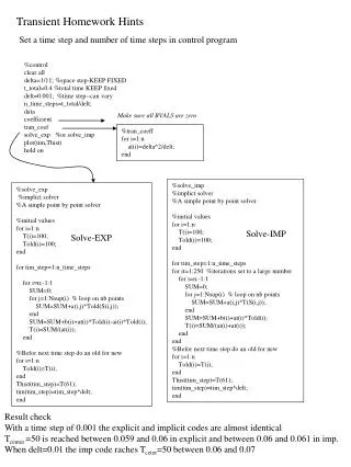
Transient Homework Hints Set a time step and number of time steps in control program %control clear all delta=1/11; %space step-KEEP FIXED t_total=0.4 %total time KEEP fixed delt=0.001; %time step--can vary n_time_steps=t_total/delt; data coefficient tran_coef solve_exp %or solve_imp plot(tim,Thist) hold on Make sure all BVALS are zero %tran_coeff for i=1:n at(i)=delta^2/delt; end %solve_imp %implict solver %A simple point by point solver %initial values for i=1:n T(i)=100; Told(i)=100; end for tim_step=1:n_time_steps for it=1:250 %iterations set to a large number for i=n:-1:1 SUM=0; for j=1:Nsup(i) % loop on nb points SUM=SUM+a(i,j)*T(S(i,j)); end SUM=SUM+b(i)+at(i)*Told(i); T(i)=SUM/(ai(i)+at(i)); end end %Befor next time step do an old for new for i=1:n Told(i)=T(i); end Thist(tim_step)=T(61); tim(tim_step)=tim_step*delt; end %solve_exp %implict solver %A simple point by point solver %initial values for i=1:n T(i)=100; Told(i)=100; end for tim_step=1:n_time_steps for i=n:-1:1 SUM=0; for j=1:Nsup(i) % loop on nb points SUM=SUM+a(i,j)*Told(S(i,j)); end SUM=SUM+b(i)+at(i)*Told(i)-ai(i)*Told(i); T(i)=SUM/(at(i)); end %Befor next time step do an old for new for i=1:n Told(i)=T(i); end Thist(tim_step)=T(61); tim(tim_step)=tim_step*delt; end Solve-IMP Solve-EXP Result check With a time step of 0.001 the explicit and implicit codes are almost identical Tcenter =50 is reached between 0.059 and 0.06 in explicit and between 0.06 and 0.061 in imp. When delt=0.01 the imp code raches Tceter=50 between 0.06 and 0.07