Implementing Transient Heat Transfer Analysis with Explicit and Implicit Methods
This guide provides step-by-step instructions for implementing a transient heat transfer analysis using both explicit and implicit methods in a control program. The process involves defining time steps, the total duration, and coefficients for numerical stability. Key components include setting initial values, iterating through time steps, and comparing results from explicit and implicit solvers. The implementation allows users to check convergence by analyzing how closely the center temperature approaches a target value. Suitable for educational and practical applications in thermal analysis.

Implementing Transient Heat Transfer Analysis with Explicit and Implicit Methods
E N D
Presentation Transcript
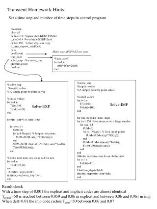
Transient Homework Hints Set a time step and number of time steps in control program %control clear all delta=1/11; %space step-KEEP FIXED t_total=0.4 %total time KEEP fixed delt=0.001; %time step--can vary n_time_steps=t_total/delt; data coefficient tran_coef solve_exp %or solve_imp plot(tim,Thist) hold on Make sure all BVALS are zero %tran_coeff for i=1:n at(i)=delta^2/delt; end %solve_imp %implict solver %A simple point by point solver %initial values for i=1:n T(i)=100; Told(i)=100; end for tim_step=1:n_time_steps for it=1:250 %iterations set to a large number for i=n:-1:1 SUM=0; for j=1:Nsup(i) % loop on nb points SUM=SUM+a(i,j)*T(S(i,j)); end SUM=SUM+b(i)+at(i)*Told(i); T(i)=SUM/(ai(i)+at(i)); end end %Befor next time step do an old for new for i=1:n Told(i)=T(i); end Thist(tim_step)=T(61); tim(tim_step)=tim_step*delt; end %solve_exp %implict solver %A simple point by point solver %initial values for i=1:n T(i)=100; Told(i)=100; end for tim_step=1:n_time_steps for i=n:-1:1 SUM=0; for j=1:Nsup(i) % loop on nb points SUM=SUM+a(i,j)*Told(S(i,j)); end SUM=SUM+b(i)+at(i)*Told(i)-ai(i)*Told(i); T(i)=SUM/(at(i)); end %Befor next time step do an old for new for i=1:n Told(i)=T(i); end Thist(tim_step)=T(61); tim(tim_step)=tim_step*delt; end Solve-IMP Solve-EXP Result check With a time step of 0.001 the explicit and implicit codes are almost identical Tcenter =50 is reached between 0.059 and 0.06 in explicit and between 0.06 and 0.061 in imp. When delt=0.01 the imp code raches Tceter=50 between 0.06 and 0.07