Lower Bounds for Comparison-Based Sorting Algorithms (Ch. 8)

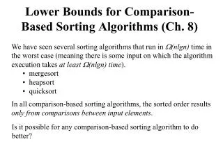
Lower Bounds for Comparison-Based Sorting Algorithms (Ch. 8) • We have seen several sorting algorithms that run in (nlgn) time in • the worst case (meaning there is some input on which the algorithm • execution takes at least (nlgn) time). • mergesort • heapsort • quicksort In all comparison-based sorting algorithms, the sorted order results only from comparisons between input elements. Is it possible for any comparison-based sorting algorithm to do better?

Lower Bounds for Sorting Algorithms Theorem: Any comparison-based sort must make (nlgn) comparisons in the worst case to sort a sequence of n elements. But how do we prove this? We'll use the decision tree model to represent any sorting algorithm and then argue that no matter the algorithm, there is some input that will cause it to run in (nlgn) time.

The Decision Tree Model • Given any comparison-based sorting algorithm, we can represent • its behavior on an input of size n by a decision tree. Note: we need • only consider the comparisons in the algorithm (the other operations • only make the algorithm take longer). • each internal node in the decision tree corresponds to one of the comparisons in the algorithm. • start at the root and do first comparison: - if  take left branch, if > take right branch, etc. • each leaf represents one possible ordering of the input - one leaf for each of n! possible orderings.  One decision tree exists for each algorithm and input size

A[1] vs A[2] A[2] vs A[3] A[1] vs A[3] A[1] vs A[3] A[2] vs A[3] A[2], A[3], A[1] A[3], A[2], A[1] A[1], A[2], A[3] A[1], A[3], A[2] A[3], A[1], A[2] A[2], A[1], A[3] The Decision Tree Model Example: Insertion sort with n = 3 (3! = 6 leaves)  >  > >    > > Note: The length of the longest root to leaf path in this tree = worst-case number of comparisons  worst-case number of operations of algorithm

The (nlgn) Lower Bound Theorem: Any decision tree T for sorting n elements has height (nlgn) (therefore, any comparison sort algorithm requires (nlgn) compares in the worst case). • Proof: Let h be the height of T. Then we know • T has at least n! leaves • T is binary, so it has at most 2h leaves n!  #leaves  2h 2h  n! lg(2h)  lg(n!) h  (nlgn) (Eq. 3.18) 

Beating the lower bound ...non-comparison based sorts Idea: Algorithms that are NOT comparison based might be faster. • There are three such algorithms presented in Chapter 8: • counting sort • radix sort • bucket sort • These algorithms • run in O(n) time (if certain conditions can be guaranteed) • either use information about the values to be sorted (counting sort, bucket sort), or • operate on "pieces" of the input elements (radix sort)

Counting Sort Requirement: input elements are integers in known range [0..k] for some constant k. Idea:for each input element x, find the number of elements x (say this number = m) and put x in the (m+1)st spot in the output array. • Counting-Sort(A, k) • // A[1..n] is input array, C[0..k] is initially all 0's, B[1..n] is output array 1. for i  1 to length(A) do 2. C[A[i]]  C[A[i]] + 1 3. for i  1 to k do 4. C[i]  C[i] + C[i-1] // Make C into a "prefix sum" array, where C[i] // contains number of elements  i • 5. for j length(A) downto 1 do • 6. B[C[A[j]]]  A[j] 7. C[A[j]] C[A[j]] - 1

Running Time of Counting Sort for loop in lines 1-2 takes (n) time. for loop in lines 3-4 takes (k) time. for loop in lines 5-7 takes (n) time. In practice, use counting sort when we have k = (n), so running time is (n). Counting sort has the important property of stability: A sorting algorithm is stable when numbers with the same values appear in the output array in the same order as they do in the input array. Important when satellite data is stored with elements being sorted and when counting sort is used as a subroutine for radix sort. Overall time is (k + n).

Radix Sort Let d be the number of digits in each input number. • Radix-Sort(A, d) • 1. fori 1 toddo • 2. use stable sort to sort array A on digit i • Note: • radix sort sorts the least significant digit first. • correctness can be shown by induction on the digit being sorted. • often counting sort is used as the internal sort in step 2.

Radix Sort Let d be the number of digits in each input number. • Radix-Sort(A, d) • 1. fori 1 toddo • 2. use stable sort to sort array A on digit i • Running time of radix sort:O(dTss(n)) • Tss is the time for the internal sort. Counting sort gives Tss(n) = O(k + n), so O(dTss(n)) = O(d(k + n)), which is O(n) if d = O(1) and k = O(n). • if d = O(lgn) and k = 2 (common for computers), then O(d(k+n)) = O(nlgn)

Bucket Sort Assumption: input elements distributed uniformly over some known range, e.g., [0,1), so all elements in A are greater than or equal to 0 but less than 1 . (Appendix C.2 has defn of uniform distribution) • Bucket-Sort(A) • 1. n = length[A] 2. for i = 1 to n • do insert A[i] into list B[floor of nA[i]] 4. for i = 0 to n-1 • do sort list i with Insertion-Sort • 6. Concatenate lists B[0], B[1],…,B[n-1]

Bucket Sort • Bucket-Sort(A, x, y) • 1. divide interval [x, y) into n equal-sized subintervals (buckets) 2. distribute the n input keys into the buckets 3. sort the numbers in each bucket (e.g., with insertion sort) 4. scan the (sorted) buckets in order and produce output array Running time of bucket sort:O(n) expected time Step 1: O(1) for each interval = O(n) time total. Step 2: O(n) time. Step 3: The expected number of elements in each bucket is O(1) (see book for formal argument, section 8.4), so total is O(n) Step 4:O(n) time to scan the n buckets containing a total of n input elements

Summary NCB Sorts Non-Comparison Based Sorts Running Time worst-case average-case best-case in place Counting Sort O(n + k) O(n + k) O(n + k) no Radix Sort O(d(n + k')) O(d(n + k')) O(d(n + k')) no Bucket Sort O(n) no Counting sort assumes input elements are in range [0,1,2,..,k] and uses array indexing to count the number of occurrences of each value. Radix sort assumes each integer consists of d digits, and each digit is in range [1,2,..,k']. Bucket sort requires advance knowledge of input distribution (sorts n numbers uniformly distributed in range in O(n) time).

Lower Bounds for Comparison-Based Sorting Algorithms (Ch. 8)