Parallel Graph Algorithms
Parallel Graph Algorithms. Kamesh Madduri KMadduri@lbl.gov. Talk Outline. Applications Parallel algorithm building blocks Kernels Data structures Parallel algorithm case studies Connected components BFS/Shortest paths Betweenness Centrality Performance on current systems Software

Parallel Graph Algorithms
E N D
Presentation Transcript
Parallel Graph Algorithms KameshMadduri KMadduri@lbl.gov
Talk Outline • Applications • Parallel algorithm building blocks • Kernels • Data structures • Parallel algorithm case studies • Connected components • BFS/Shortest paths • Betweenness Centrality • Performance on current systems • Software • Architectures • Performance trends Parallel Graph Algorithms
Routing in transportation networks Road networks, Point-to-point shortest paths: 15 seconds (naïve) 10 microseconds H. Bast et al., “Fast Routing in Road Networks with Transit Nodes”,Science 27, 2007. Parallel Graph Algorithms
Internet and the WWW • The world-wide web can be represented as a directed graph • Web search and crawl: traversal • Link analysis, ranking: Page rank and HITS • Document classification and clustering • Internet topologies (router networks) are naturally modeled as graphs Parallel Graph Algorithms
Scientific Computing • Reorderings for sparse solvers • Fill reducing orderings • partitioning, traversals, eigenvectors • Heavy diagonal to reduce pivoting (matching) • Data structures for efficient exploitation of sparsity • Derivative computations for optimization • Matroids, graph colorings, spanning trees • Preconditioning • Incomplete Factorizations • Partitioning for domain decomposition • Graph techniques in algebraic multigrid • Independent sets, matchings, etc. • Support Theory • Spanning trees & graph embedding techniques B. Hendrickson, “Graphs and HPC: Lessons for Future Architectures”,http://www.er.doe.gov/ascr/ascac/Meetings/Oct08/Hendrickson%20ASCAC.pdf Parallel Graph Algorithms
Large-scale data analysis • Graph abstractions are very useful to analyze complex data sets. • Sources of data: petascale simulations, experimental devices, the Internet, sensor networks • Challenges: data size, heterogeneity, uncertainty, data quality Social Informatics: new analytics challenges, data uncertainty Astrophysics: massive datasets, temporal variations Bioinformatics: data quality, heterogeneity Image sources: (1) http://physics.nmt.edu/images/astro/hst_starfield.jpg (2,3) www.visualComplexity.com Parallel Graph Algorithms
Data Analysis and Graph Algorithms in Systems Biology • Study of the interactions between various components in a biological system • Graph-theoretic formulations are pervasive: • Predicting new interactions: modeling • Functional annotation of novel proteins: matching, clustering • Identifying metabolic pathways: paths, clustering • Identifying new protein complexes: clustering, centrality Image Source: Giot et al., “A Protein Interaction Map of Drosophila melanogaster”, Science 302, 1722-1736, 2003. Parallel Graph Algorithms
Graph –theoretic problems in social networks • Community identification: clustering • Targeted advertising: centrality • Information spreading: modeling Image Source: Nexus (Facebook application) Parallel Graph Algorithms
Network Analysis for Intelligence and Survelliance • [Krebs ’04] Post 9/11 Terrorist Network Analysis from public domain information • Plot masterminds correctly identified from interaction patterns: centrality • A global view of entities is often more insightful • Detect anomalous activities by exact/approximate graph matching Image Source: http://www.orgnet.com/hijackers.html Image Source: T. Coffman, S. Greenblatt, S. Marcus, Graph-based technologies for intelligence analysis, CACM, 47 (3, March 2004): pp 45-47 Parallel Graph Algorithms
Characterizing Graph-theoretic computations Factors that influence choice of algorithm Input: Graph abstraction Graph kernel • graph sparsity (m/n ratio) • static/dynamic nature • weighted/unweighted, weight distribution • vertex degree distribution • directed/undirected • simple/multi/hyper graph • problem size • granularity of computation at nodes/edges • domain-specific characteristics • traversal • shortest path algorithms • flow algorithms • spanning tree algorithms • topological sort • ….. Problem: Find *** • paths • clusters • partitions • matchings • patterns • orderings Graph problems are often recast as sparse linear algebra (e.g., partitioning) or linear programming (e.g., matching) computations Parallel Graph Algorithms
Talk Outline • Applications • Parallel algorithm building blocks • Kernels • Data structures • Parallel algorithm case studies • Connected components • BFS/Shortest paths • Betweenness centrality • Performance on current systems • Software • Architectures • Performance trends Parallel Graph Algorithms
Parallel Computing Models: A Quick PRAM review • Objectives • Bridge between software and hardware • General purpose HW, scalable HW • Transportable SW • Abstract architecture for algorithm development • Why is it so important? • Uniprocessor: von Neumann model of computation • Parallel processors Multicore • Requirements: inherent tension • Simplicity to make analysis of interesting problems tractable • Detailed to reveal the important bottlenecks • Models, e.g.: • PRAM: rich collection of parallel graph algorithms • BSP: some CGM algorithms (cgmGraph) • LogP Parallel Graph Algorithms
PRAM • Ideal model of a parallel computer for analyzing the efficiency of parallel algorithms. • PRAM composed of • P unmodifiable programs, each composed of optionally labeled instructions. • a single shared memory composed of a sequence of words, each capable of containing an arbitrary integer. • P accumulators, one associated with each program • a read-only input tape • a write-only output tape • No local memory in each RAM. • Synchronization, communication, parallel overhead is zero. Parallel Graph Algorithms
PRAM Data Access Forms • EREW (Exclusive Read, Exclusive Write) • A memory cell can be read or written by at most one processor per cycle. • Ensures no read or write conflicts. • CREW (Concurrent Read, Exclusive Write) • Ensures there are no write conflicts. • CRCW (Concurrent Read, Concurrent Write) • Requires use of some conflict resolution scheme. Parallel Graph Algorithms
PRAM Pros and Cons • Pros • Simple and clean semantics. • The majority of theoretical parallel algorithms are specified with the PRAM model. • Independent of the communication network topology. • Cons • Not realistic, too powerful communication model. • Algorithm designer is misled to use IPC without hesitation. • Synchronized processors. • No local memory. • Big-O notation is often misleading. Parallel Graph Algorithms
Analyzing Parallel Graph Algorithms • Problem parameters: n, m, D (graph diameter) • Worst-case running time: T • Total number of operations (work): W • Nick’s Class (NC): complexity class for problems that can be solved in poly-logarithmic time using a polynomial number of processors • P-complete: inherently sequential Parallel Graph Algorithms
The Helman-JaJa model • Extension to the PRAM model for shared memory algorithm design and analysis. • T(n, p) is measured by the triplet –TM(n, p), TC(n, p), B(n, p) • TM(n, p): maximum number of non-contiguous main memory accesses required by any processor • TC(n, p): upper bound on the maximum local computational complexity of any of the processors • B(n, p): number of barrier synchronizations. Parallel Graph Algorithms
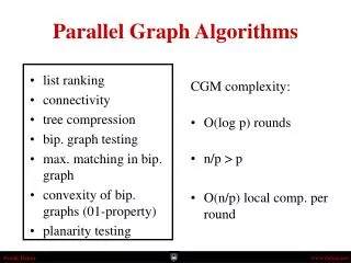
Building blocks of classical PRAM graph algorithms • Prefix sums • List ranking • Euler tours, Pointer jumping, Symmetry breaking • Sorting • Tree contraction Parallel Graph Algorithms
Prefix Sums • Input: A, an array of n elements; associative binary operation • Output: • O(n) work, O(log n) time, • n processors B(3,1) C(3,2) B(2,2) C(2,2) B(2,1) C(2,1) B(1,3) C(1,3) B(1,4) C(1,4) B(1,2) C(1,2) B(1,1) C(1,1) B(0,1) C(0,1) B(0,2) C(0,2) B(0,3) C(0,3) B(0,4) C(0,4) B(0,5) C(0,5) B(0,6) C(0,6) B(0,7) C(0,7) B(0,8) C(0,8) Parallel Graph Algorithms
Parallel Prefix • X: array of n elements stored in arbitrary order. • For each element i, let X(i).value be its value and X(i).next be the index of its successor. • For binary associative operator Θ, compute X(i).prefix such that • X(head).prefix = X (head).value, and • X(i).prefix = X(i).value Θ X(predecessor).prefix where • head is the first element • i is not equal to head, and • predecessor is the node preceding i. • List ranking: special case of parallel prefix, values initially set to 1, and addition is the associative operator. Parallel Graph Algorithms
List ranking Illustration • Ordered list (X.next values) • Random list (X.next values) 8 9 5 6 7 2 3 4 2 9 7 8 3 4 6 5 Parallel Graph Algorithms
List Ranking key idea 1. Chop X randomly into s pieces 2. Traverse each piece using a serial algorithm. 3. Compute the global rank of each element using the result computed from the second step. • Locality (list ordering) determines performance • In the Helman-JaJa model, TM(n,p) = O(n/p). Parallel Graph Algorithms
An example higher-level algorithm Tarjan-Vishkin’sbiconnected components algorithm: O(log n) time, O(m+n) time. • Compute spanning tree T for the input graph G. • Compute Eulerian circuit for T. • Root the tree at an arbitrary vertex. • Preorder numbering of all the vertices. • Label edges using vertex numbering • Connected components using the Shiloach-Vishkin algorithm Parallel Graph Algorithms
Data structures: graph representation • Dense graphs (m = O(n2)): adjacency matrix commonly used. • Sparse graphs: adjacency lists, similar to the CSR matrix format. • Dynamic sparse graphs: we need to support edge and vertex membership queries, insertions, and deletions. • should be space-efficient, with low synchronization overhead • Several different representations possible • Resizable adjacency arrays • Adjacency arrays, sorted by vertex identifiers • Adjacency arrays for low-degree vertices, heap-based structures for high-degree vertices (for sparse graphs with skewed degree distributions) Parallel Graph Algorithms
Data structures in (Parallel) Graph Algorithms • A wide range of ADTs in graph algorithms: array, list, queue, stack, set, multiset, tree • ADT implementations are typically array-based for performance considerations. • Key data structure considerations in parallel graph algorithm design • Practical parallel priority queues • Space-efficiency • Parallel set/multiset operations, e.g., union, intersection, etc. Parallel Graph Algorithms
Talk Outline • Applications • Parallel algorithm building blocks • Kernels • Data structures • Parallel algorithm case studies • Connected components • BFS/Shortest paths • Betweenness centrality • Performance on current systems • Software • Architectures • Performance trends Parallel Graph Algorithms
Connected Components • Building blocks for many graph algorithms • Minimum spanning tree, spanning tree, planarity testing, etc. • Representative of the “graft-and-shortcut” approach • CRCW PRAM algorithms • [Shiloach & Vishkin ’82]: O(log n) time, O((m+n) logn) work • [Gazit ’91]: randomized, optimal, O(log n) time. • CREW algorithms – [Han & Wagner ’90]: O(log2n) time, O((m+nlog n) logn) work. Parallel Graph Algorithms
Shiloach-Vishkin algorithm • Input: n isolated vertices and m PRAM processors. • Each processor Pigrafts a tree rooted at vertex vito the tree that contains one of its neighbors u under the constraints u< vi • Grafting creates k ≥ 1 connected subgraphs, and each subgraph is then shortcut so that the depth of the trees reduce at least by half. • Repeat graft and shortcut until no more grafting is possible. • Runs on arbitrary CRCW PRAM in O(logn) time with O(m) processors. • Helman-JaJa model: TM = (3m/p + 2)log n, TB = 4log n. Parallel Graph Algorithms
SV pseudo-code • Input: (1) A set of m edges (i, j) given in arbitrary order. (2) Array D[1..n] with D[i] = i • Output: Array D[1..n] with D[i] being the component to which vertex i belongs. begin while true do 1. for (i, j) ∈ E in parallel do if D[i]=D[D[i]] and D[j]<D[i] thenD[D[i]] = D[j]; 2. for (i, j) ∈ E in parallel do if i belongs to a star and D[j]=D[i] thenD[D[i]] = D[j]; 3. if all vertices are in rooted stars then exit; for all i in parallel do D[i] = D[D[i]] end Parallel Graph Algorithms
SV Illustration 2 2 4 4 1st iter 2,3 1,4 3 3 1 1 shortcut Input graph graft 2nd iter 1 1 2 1 2 Parallel Graph Algorithms
Talk Outline • Applications • Parallel algorithm building blocks • Kernels • Data structures • Parallel algorithm case studies • Connected components • BFS/Shortest paths • Betweenness centrality • Performance on current systems • Software • Architectures • Performance trends Parallel Graph Algorithms
Parallel Single-source Shortest Paths (SSSP) algorithms • No known PRAM algorithm that runs in sub-linear time and O(m+nlog n) work • Parallel priority queues: relaxed heaps [DGST88], [BTZ98] • Ullman-Yannakakis randomized approach [UY90] • Meyer et al. ∆ - stepping algorithm [MS03] • Distributed memory implementations based on graph partitioning • Heuristics for load balancing and termination detection K. Madduri, D.A. Bader, J.W. Berry, and J.R. Crobak, “An Experimental Study of A Parallel Shortest Path Algorithm for Solving Large-Scale Graph Instances,” Workshop on Algorithm Engineering and Experiments (ALENEX), New Orleans, LA, January 6, 2007. Parallel Graph Algorithms
∆ - stepping algorithm [MS03] • Label-correcting algorithm: Can relax edges from unsettled vertices also • ∆ - stepping: “approximate bucket implementation of Dijkstra’s algorithm” • ∆: bucket width • Vertices are ordered using buckets representing priority range of size ∆ • Each bucket may be processed in parallel Parallel Graph Algorithms
Classify edges as “heavy” and “light” Parallel Graph Algorithms
Relax light edges (phase) Repeat until B[i] Is empty Parallel Graph Algorithms
Relax heavy edges. No reinsertions in this step. Parallel Graph Algorithms
∆ - stepping algorithm: illustration ∆ = 0.1 (say) 0.05 • One parallel phase • while (bucket is non-empty) • Inspect light edges • Construct a set of “requests” (R) • Clear the current bucket • Remember deleted vertices (S) • Relax request pairs in R • Relax heavy request pairs (from S) • Go on to the next bucket 0.56 3 6 0.07 0.01 0.15 0.23 4 2 0 0.02 0.13 0.18 5 1 d array 0 1 2 3 4 5 6 ∞ ∞ ∞ ∞ ∞ ∞ ∞ Buckets Parallel Graph Algorithms
∆ - stepping algorithm: illustration 0.05 • One parallel phase • while (bucket is non-empty) • Inspect light edges • Construct a set of “requests” (R) • Clear the current bucket • Remember deleted vertices (S) • Relax request pairs in R • Relax heavy request pairs (from S) • Go on to the next bucket 0.56 3 6 0.07 0.01 0.15 0.23 4 2 0 0.02 0.13 0.18 5 1 d array 0 1 2 3 4 5 6 ∞ ∞ ∞ ∞ ∞ ∞ 0 Buckets Initialization: Insert s into bucket, d(s) = 0 0 0 Parallel Graph Algorithms
∆ - stepping algorithm: illustration • One parallel phase • while (bucket is non-empty) • Inspect light edges • Construct a set of “requests” (R) • Clear the current bucket • Remember deleted vertices (S) • Relax request pairs in R • Relax heavy request pairs (from S) • Go on to the next bucket 0.05 0.56 3 6 0.07 0.01 0.15 0.23 4 2 0 0.02 0.13 0.18 5 1 d array 0 1 2 3 4 5 6 ∞ ∞ ∞ ∞ ∞ ∞ 0 R 2 Buckets 0 0 .01 S Parallel Graph Algorithms
∆ - stepping algorithm: illustration 0.05 • One parallel phase • while (bucket is non-empty) • Inspect light edges • Construct a set of “requests” (R) • Clear the current bucket • Remember deleted vertices (S) • Relax request pairs in R • Relax heavy request pairs (from S) • Go on to the next bucket 0.56 3 6 0.07 0.01 0.15 0.23 4 2 0 0.02 0.13 0.18 5 1 d array 0 1 2 3 4 5 6 ∞ ∞ ∞ ∞ ∞ ∞ 0 2 Buckets R 0 .01 0 S Parallel Graph Algorithms
∆ - stepping algorithm: illustration 0.05 • One parallel phase • while (bucket is non-empty) • Inspect light edges • Construct a set of “requests” (R) • Clear the current bucket • Remember deleted vertices (S) • Relax request pairs in R • Relax heavy request pairs (from S) • Go on to the next bucket 0.56 3 6 0.07 0.01 0.15 0.23 4 2 0 0.02 0.13 0.18 5 1 d array 0 1 2 3 4 5 6 ∞ ∞ ∞ ∞ ∞ 0 .01 R Buckets 0 2 0 S Parallel Graph Algorithms
∆ - stepping algorithm: illustration 0.05 • One parallel phase • while (bucket is non-empty) • Inspect light edges • Construct a set of “requests” (R) • Clear the current bucket • Remember deleted vertices (S) • Relax request pairs in R • Relax heavy request pairs (from S) • Go on to the next bucket 0.56 3 6 0.07 0.01 0.15 0.23 4 2 0 0.02 0.13 0.18 5 1 d array 0 1 2 3 4 5 6 ∞ ∞ ∞ ∞ ∞ 0 .01 Buckets R 1 3 0 2 .03 .06 0 S Parallel Graph Algorithms
∆ - stepping algorithm: illustration 0.05 • One parallel phase • while (bucket is non-empty) • Inspect light edges • Construct a set of “requests” (R) • Clear the current bucket • Remember deleted vertices (S) • Relax request pairs in R • Relax heavy request pairs (from S) • Go on to the next bucket 0.56 3 6 0.07 0.01 0.15 0.23 4 2 0 0.02 0.13 0.18 5 1 d array 0 1 2 3 4 5 6 ∞ ∞ ∞ ∞ ∞ 0 .01 R Buckets 1 3 0 .03 .06 S 0 2 Parallel Graph Algorithms
∆ - stepping algorithm: illustration 0.05 • One parallel phase • while (bucket is non-empty) • Inspect light edges • Construct a set of “requests” (R) • Clear the current bucket • Remember deleted vertices (S) • Relax request pairs in R • Relax heavy request pairs (from S) • Go on to the next bucket 0.56 3 6 0.07 0.01 0.15 0.23 4 2 0 0.02 0.13 0.18 5 1 d array 0 1 2 3 4 5 6 ∞ ∞ ∞ 0 .03 .01 .06 Buckets R 3 0 1 S 0 2 Parallel Graph Algorithms
∆ - stepping algorithm: illustration 0.05 • One parallel phase • while (bucket is non-empty) • Inspect light edges • Construct a set of “requests” (R) • Clear the current bucket • Remember deleted vertices (S) • Relax request pairs in R • Relax heavy request pairs (from S) • Go on to the next bucket 0.56 3 6 0.07 0.01 0.15 0.23 4 2 0 0.02 0.13 0.18 5 1 d array 0 1 2 3 4 5 6 0 .29 .03 .01 .06 .16 .62 Buckets R 1 4 2 5 S 0 1 3 2 6 6 Parallel Graph Algorithms
No. of phases (machine-independent performance count) high diameter low diameter Parallel Graph Algorithms
Average shortest path weight for various graph families~ 220 vertices, 222 edges, directed graph, edge weights normalized to [0,1] Parallel Graph Algorithms
Last non-empty bucket (machine-independent performance count) Fewer buckets, more parallelism Parallel Graph Algorithms
Number of bucket insertions (machine-independent performance count) Parallel Graph Algorithms