Graph Searching Algorithms
Learn about graph representation, graph searching methods like Breadth-First Search (BFS) and Depth-First Search (DFS), with code examples for BFS, properties of BFS, and Depth-First Search exploration strategy.

Graph Searching Algorithms
E N D
Presentation Transcript
Graph Algorithms Searching
Review: Graphs • A graph G = (V, E) • V = set of vertices, E = set of edges • Densegraph: |E| |V|2; Sparse graph: |E| |V| • Undirected graph: • Edge (u,v) = Edge (v,u) • No self-loops • Directed graph: • Edge (u,v) goes from vertex u to vertex v, notated uv • A weighted graph associates weights with either the edges or the vertices
Review: Representing Graphs • Assume V = {1, 2, …, n} • An adjacency matrixrepresents the graph as a n x n matrix A: • A[i, j] = 1 if edge (i, j) E (or weight of edge) = 0 if edge (i, j) E • Storage requirements: O(|V|2) • A dense representation • An adjacency list represents the graph as n lists of adjacent vertices • Storage requirements: O(|V| + |E|)
Graph Searching • Given: a graph G = (V, E), directed or undirected • Goal: methodically explore every vertex and every edge • Ultimately: build a tree on the graph • Pick a vertex as the root (origin of search) • Choose certain edges to produce a tree • Note: might also build a forest if graph is not connected
Breadth-First Search • “Explore” a graph, turning it into a tree • One vertex at a time • Expand frontier of explored vertices across the breadth of the frontier • Builds a tree over the graph • Pick a source vertex to be the root • Find (“discover”) its children, then their children, etc.
Breadth-First Search • Associate vertex “colors” to guide the algorithm • White vertices have not been discovered • All vertices start out white • Grey vertices are discovered but not fully explored • They are enqueued • Black vertices are discovered and fully explored • They are adjacent only to black and gray vertices • Fully explored adjacency list fully processed • Explore vertices by scanning adjacency list of grey vertices
Breadth-First Search BFS(G, s) { initialize vertices; // (For all v) [ v->color = WHITE, v->d = INF ] // s->color = GREY, s->d = 0 Q = {s}; // Q is a queue; initialize to s while (Q not empty) { u = RemoveFront(Q); for each v u->Adj[] { if (v->color == WHITE) v->color = GREY; v->d = u->d + 1; v->p = u; Enqueue(Q, v); } u->color = BLACK; } } What does v->d represent? What does v->p represent?
Breadth-First Search: Example r s t u v w x y
Breadth-First Search: Example r s t u 0 v w x y Front Q: s
Breadth-First Search: Example r->p = s r s t u 1 0 1 v w x y Q: w r
Breadth-First Search: Example r s t u 1 0 2 1 2 v w x y Q: r t x
Breadth-First Search: Example r s t u 1 0 2 2 1 2 v w x y Q: t x v
Breadth-First Search: Example r s t u 1 0 2 3 2 1 2 v w x y Q: x v u
Breadth-First Search: Example r s t u 1 0 2 3 2 1 2 3 v w x y Q: v u y
Breadth-First Search: Example r s t u 1 0 2 3 2 1 2 3 v w x y Q: u y
Breadth-First Search: Example r s t u 1 0 2 3 2 1 2 3 v w x y Q: y
Breadth-First Search: Example r s t u 1 0 2 3 2 1 2 3 v w x y Q: Ø
Touch every vertex: O(V) u = every vertex, but only once (Why?) So v = every vertex that appears in some other vert’s adjacency list BFS: The Code Again BFS(G, s) { initialize vertices; Q = {s}; while (Q not empty) { u = RemoveTop(Q); for each v u->Adj[] { if (v->color == WHITE) v->color = GREY; v->d = u->d + 1; v->p = u; Enqueue(Q, v); } u->color = BLACK; } } What will be the running time? Total running time: O(V+E)
BFS: The Code Again BFS(G, s) { initialize vertices; Q = {s}; while (Q not empty) { u = RemoveTop(Q); for each v u->Adj[] { if (v->color == WHITE) v->color = GREY; v->d = u->d + 1; v->p = u; Enqueue(Q, v); } u->color = BLACK; } }
Breadth-First Search: Properties • BFS calculates the shortest-path distance to the source node • Shortest-path distance (s,v) = minimum number of edges from s to v, or if v not reachable from s • BFS builds breadth-first tree, in which paths to root represent shortest paths in G • Thus can use BFS to calculate shortest path from one vertex to another in O(V+E) time
Depth-First Search • Depth-first search is another strategy for exploring a graph • Explore “deeper” in the graph whenever possible • Edges are explored out of most recently discovered vertex v that still has unexplored edges • When all of v’s edges have been explored, backtrack to vertex from which v was discovered
Depth-First Search • Vertices initially colored white • Then colored gray when discovered • Then black when finished
DFS(G) { for each vertex u G->V { u->color = WHITE; } time = 0; for each vertex u G->V { if (u->color == WHITE) DFS_Visit(u); } } DFS_Visit(u) { u->color = GREY; ++time; u->d = time; for each v u->Adj[] { if (v->color == WHITE) DFS_Visit(v); } u->color = BLACK; ++time; u->f = time; } Depth-First Search: Code
DFS(G) { for each vertex u G->V { u->color = WHITE; } time = 0; for each vertex u G->V { if (u->color == WHITE) DFS_Visit(u); } } DFS_Visit(u) { u->color = GREY; ++time; u->d = time; for each v u->Adj[] { if (v->color == WHITE) DFS_Visit(v); } u->color = BLACK; ++time; u->f = time; } Depth-First Search: Code What does u->d represent?
DFS(G) { for each vertex u G->V { u->color = WHITE; } time = 0; for each vertex u G->V { if (u->color == WHITE) DFS_Visit(u); } } DFS_Visit(u) { u->color = GREY; ++time; u->d = time; for each v u->Adj[] { if (v->color == WHITE) DFS_Visit(v); } u->color = BLACK; ++time; u->f = time; } Depth-First Search: Code What does u->f represent?
DFS(G) { for each vertex u G->V { u->color = WHITE; } time = 0; for each vertex u G->V { if (u->color == WHITE) DFS_Visit(u); } } DFS_Visit(u) { u->color = GREY; ++time; u->d = time; for each v u->Adj[] { if (v->color == WHITE) DFS_Visit(v); } u->color = BLACK; ++time; u->f = time; } Depth-First Search: Code Will all vertices eventually be colored black?
DFS(G) { for each vertex u G->V { u->color = WHITE; } time = 0; for each vertex u G->V { if (u->color == WHITE) DFS_Visit(u); } } DFS_Visit(u) { u->color = GREY; ++time; u->d = time; for each v u->Adj[] { if (v->color == WHITE) DFS_Visit(v); } u->color = BLACK; ++time; u->f = time; } Depth-First Search: Code What will be the running time?
DFS(G) { for each vertex u G->V { u->color = WHITE; } time = 0; for each vertex u G->V { if (u->color == WHITE) DFS_Visit(u); } } DFS_Visit(u) { u->color = GREY; ++time; u->d = time; for each v u->Adj[] { if (v->color == WHITE) DFS_Visit(v); } u->color = BLACK; ++time; u->f = time; } Depth-First Search: Code Running time: O(n2) because call DFS_Visit on each vertex, and the loop over Adj[] can run as many as |V| times
DFS(G) { for each vertex u G->V { u->color = WHITE; } time = 0; for each vertex u G->V { if (u->color == WHITE) DFS_Visit(u); } } DFS_Visit(u) { u->color = GREY; ++time; u->d = time; for each v u->Adj[] { if (v->color == WHITE) DFS_Visit(v); } u->color = BLACK; ++time; u->f = time; } Depth-First Search: Code BUT, there is actually a tighter bound. How many times will DFS_Visit() actually be called?
DFS(G) { for each vertex u G->V { u->color = WHITE; } time = 0; for each vertex u G->V { if (u->color == WHITE) DFS_Visit(u); } } DFS_Visit(u) { u->color = GREY; ++time; u->d = time; for each v u->Adj[] { if (v->color == WHITE) DFS_Visit(v); } u->color = BLACK; ++time; u->f = time; } Depth-First Search: Code So, running time of DFS = O(V+E)
Depth-First Sort Analysis • This running time argument is an informal example of amortized analysis • “Charge” the exploration of edge to the edge • Each loop in DFS_Visit can be attributed to an edge in the graph • Runs once/edge if directed graph, twice if undirected • Thus loop will run in O(E) time, algorithm O(V+E) • Considered linear for graph, b/c adj list requires O(V+E) storage
DFS Example sourcevertex
DFS Example sourcevertex d f 1 | | | | | | | |
DFS Example sourcevertex d f 1 | | | 2 | | | | |
DFS Example sourcevertex d f 1 | | | 2 | | 3 | | |
DFS Example sourcevertex d f 1 | | | 2 | | 3 | 4 | |
DFS Example sourcevertex d f 1 | | | 2 | | 3 | 4 5 | |
DFS Example sourcevertex d f 1 | | | 2 | | 3 | 4 5 | 6 |
DFS Example sourcevertex d f 1 | 8 | | 2 | 7 | 3 | 4 5 | 6 |
DFS Example sourcevertex d f 1 | 8 | | 2 | 7 | 3 | 4 5 | 6 |
DFS Example sourcevertex d f 1 | 8 | | 2 | 7 9 | 3 | 4 5 | 6 |
DFS Example sourcevertex d f 1 | 8 | | 2 | 7 9 |10 3 | 4 5 | 6 |
DFS Example sourcevertex d f 1 | 8 |11 | 2 | 7 9 |10 3 | 4 5 | 6 |
DFS Example sourcevertex d f 1 |12 8 |11 | 2 | 7 9 |10 3 | 4 5 | 6 |
DFS Example sourcevertex d f 1 |12 8 |11 13| 2 | 7 9 |10 3 | 4 5 | 6 |
DFS Example sourcevertex d f 1 |12 8 |11 13| 2 | 7 9 |10 3 | 4 5 | 6 14|
DFS Example sourcevertex d f 1 |12 8 |11 13| 2 | 7 9 |10 3 | 4 5 | 6 14|15
DFS Example sourcevertex d f 1 |12 8 |11 13|16 2 | 7 9 |10 3 | 4 5 | 6 14|15
DFS: Kinds of edges • DFS introduces an important distinction among edges in original graph • Tree edge: encounter new (white) vertex • Form a spanning forest • Can tree edges form cycles? Why or why not?
DFS Example sourcevertex d f 1 |12 8 |11 13|16 2 | 7 9 |10 3 | 4 5 | 6 14|15 Tree edges

