Download
1 / 20
220 likes | 526 Views
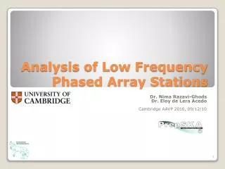
Analysis of Low Frequency Phased Array Stations . Dr. Nima Razavi-Ghods Dr. Eloy de Lera Acedo Cambridge AAVP 2010, 09/12/10. Phased array design parameters AA-lo station configuration studies (regular vs. random) Randomisation of elements Simulations to compute T A and A/T

E N D
Analysis of Low Frequency Phased Array Stations Dr. NimaRazavi-Ghods Dr. Eloy de LeraAcedo Cambridge AAVP 2010, 09/12/10
Phased array design parameters • AA-lo station configuration studies (regular vs. random) • Randomisation of elements • Simulations to compute TA and A/T (geometries, weighting, element types) • Future work and conclusions Overview
Array size (fundamental limit on Aeff/Tsys) • Array geometry (main and side-lobe profile) • Fully filled grids (regular lattice) • Sparse or thinned grids • Truly randomised grids • Antenna element response (scan/polarisation response, matching, mutual coupling) • Operating frequency, processing bandwidth, integration time • Weighting schemes (main beam and side-lobe profile) • Spatial windows (e.g. Hamming, Gaussian, Kaiser) • Side-lobe profile control (e.g. Dolph-Chebyshev/Taylor, Fourier design method) • Adaptive nulling • Back-end processing • Fully digital core (any weighting in single or multiple stages) • First level analogue (some limitations in response) Factors Affecting Beam on the Sky
Sky (Haslam) Lat = 28.59S, Long = 115.45E Date: 01/01/2020, Time 19.33h Triangular Lattice Beam 10,000 elements, d = 0.8 Random Vs. Regular
Sky (Haslam) Lat = 28.59S, Long = 115.45E Date: 01/01/2020, Time 19.33h Random Lattice Beam 10,000 elements Random Vs. Regular
d = l/3 : 2l Randomised Array: AA-lo
Variable min. distance Fixed min. distance Randomisation algorithm
TA was analysed as the beam tracked 3 cold patches on the sky over four and half hours. • Array factor based simulations carried computed using NFFT. • AA-lo Station ~10k elements. • 6 Geometries: regular, triangular, sparse random, thinned, concentric rings, and fully random. • 4 minimum inter-element separations: 0.5, 0.8, 1, 2. • 3 Weights: Uniform, Taylor and Dolph-Chebyshev (SLL = 35 dB) • 3 Element types. Simulations to compute TA
Region 1: 09h07m12s 0000’46’’, Region 2: 04h03m36s -3448’00’’ Region 3: 04h45m00s -6100’00’’ R1 R2 R3 SKA AA-lo observable Sky
Main objective: SKA simulator • Faster and more accurate simulations of the station beam based on MBF approach (collaboration with UCL). • Computation framework for station simulator (collaboration with Oxford). • Further analysis of beam synthesis techniques and weight calibration. • Design of optimal geometry, e.g. far out versus close in side-lobes. Future work and collaborations