RMS - Rainfall Runoff Modelling
DMIP-II Workshop. RMS - Rainfall Runoff Modelling. Stefan Eppert Dag Lohmann Arno Hilberts. Overview. Aim of the flood models within RMS Model structure Parameterization & Calibration Ungauged basins / uncalibrated model runs Spatial resolution, time stepping etc. Questions.

RMS - Rainfall Runoff Modelling
E N D
Presentation Transcript
DMIP-II Workshop RMS - Rainfall Runoff Modelling Stefan Eppert Dag Lohmann Arno Hilberts
Overview • Aim of the flood models within RMS • Model structure • Parameterization & Calibration • Ungauged basins / uncalibrated model runs • Spatial resolution, time stepping etc. • Questions
$ Loss Quantify Financial Loss Calculate Flood Depths Calculate Damage Define Event Stochastic Module Hazard Module Vulnerability Module Financial Module Aim of developing & using flood models in RMS • Tool for insurance industry to determine return periods for flood risks
Aim of developing & using flood models in RMS (2) • Spatial & temporal coverage Long simulation times required (~10,000 - 100,000 years) Country-wide models • Model requirements: Fast (to cover large simulation times) Flexible (to be calibrated to quite different hydrological regimes, different soil types etc.)
Soil Module Evapotranspiration Module Saturated Soil Module based on soil topographic index ETP calculated from atmospheric conditions (min data set = air temp; Ideal data set = air temp, hum, press, wind speed, net rad.) Canopy ET required for some areas State variables and fluxes • Total water deficit • Root zone water deficit • Canopy water storage • Snow water equivalent • Evapotranspiration (canopy, soil) • Throughfall (from canopy) • Runoff (Qf and Qb) • Snowmelt Runoff Routing Module Muskingum-Cunge Model Parameters • mpar = topmodel parameter • kpar = vertical water movement • fcpar = field capacity • cmpar = max. canopy water • meltpar = snow model parameter • t0par = transmissivity • rzpar = root zone depth Parameters C, X, ψcan be estimated from measured flow or river geometry Model structure dS/dt = Precipitation – Evaporation - Runoff Snow Module Partitioning of precip into rain and snow fall based on temp. (TP) above /below freezing temp. (TP0), para- meterized by two fitting parameters p1 and p2. DMIP-II: done by fitting a convolution filter (UH approach)
Model structure (2) Lumped precipitation over basin Surface runoff and baseflow from runoff generation formulas based on topographic index Flow accumulation in river channel using convolution filter
Parameterization & calibration Non-calibrated parameters (7): TP0 (freezing temp.), snow melt parameters (p1,p2), snow albedo, root zone field capacity, vertical water movement par (kpar), max. canopy storage (mcpar). 6 out of 13 are calibrated. (In previous calibrations most of the 7 fixed parameters quickly converged to values that are in accordance with textbook values).
Parameterization & calibration (2) Assume uniform prior distribution Run model for 10,000 samples, determine optimal convolution filter, and determine model ‘fit’ Create posterior distribution (grey lines) based on the ‘best performing’ 0.5% Run model for 10,000 samples, determine optimal convolution filter and pick the best performing parameter set (new posterior distribution in black)
Ungauged basins • Parameter values • Copy optimal parameter set from first gauged basin downstream. • Alternatively, copy parameter set from nearest gauged basin • Convolution filters • Same procedure, but we need to scale for basin area
Uncalibrated runs DMIP • Parameter values • Taken from an optimization conducted for the Thames, UK. • Convolution filters • Had to be ‘designed’. Assumption is that an area of 750 km2 can drain in 24 hours • Number of elements in the filter is calculated based on basin area (750 km2 = 24 elements). • Triangular shape, ‘rising limb’ stretching over 1/3 of the number of elements, ‘falling limb’ over 2/3, and sum over all elements forced to 1.
Spatial resolution & time stepping The DTMs provided are on 30x30m, which for each basin are grouped into 1000 bins/classes of topographic index values. Basin-averaged forcings are calculated based on Nexrad 4x4km data. Time stepping: hourly
Difficulties encountered… • Optimization was conducted using R2 only, allowing for large biases. • Scaling of the convolution filters is done based on upstream area, thereby disregarding river network architecture. R2 = 0.81, mean(Qobs) = 29.5 m3/s, mean(Qmod) = 11.6 m3/s