Chapter 7 Building Phylogenetic Trees

1. Chapter 7 Building Phylogenetic Trees

2. Contents • Phylogeny • Phylogenetic trees • How to make a phylogenetic tree from pairwise distances • UPGMA method (+ an example) • Neighbor-Joining method (+ an example) • Comparison of methods • Conclusion

3. Phylogeny • Phylogeny is the evolution of related species/genes • Phylogenetic tree: diagram showing evolutionary lineages of species/genes • The history of genes or species may be very different • Genes can be homologous or analogous, but still remind each other

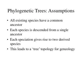
4. Phylogeny • The similarity of molecular mechanisms of the organisms that have been studied strongly suggests that all organisms on Earth had a common ancestor • Any set of species is related, and this relationship is called a phylogeny • The relationship can be represented by a phylogenetic tree

5. Phylogeny • Traditionally, morphological characters (both from living and fossilized organisms) have been used for inferring phylogenies • Zuckerkandel & Pauling (1962) showed that molecular sequences provide sets of characters that can carry a large amount information • If we have a set of sequences from different species , we may be able to use them to infer a likely phylogeny of the species in question • This assumes that the sequences have descended from some common ancestral gene in a common ancestral species

6. Phylogeny • The widespread occurrence of gene duplication means that the foregoing assumption needs to be checked carefully • The phylogentic tree of a group of seqences does not necessarily reflect the phylogenetic tree of their host species, because gene duplication is another mechanism, in addition to speciation, by which two sequences can be separated and diverge from a common ancestor • Genes which diverged because of speciation

7. Phylogeny • Genes which diverged because of speciation are called orthologues (直系同源) • Genes which diverged by gene duplication are called paralogues (平行進化同源)

8. Phylogeny • Homologous sequences can be divided into two parts • Orthologous sequences diverged by specification from a common ancestor • Paralogous sequences evolved by gene dublication within species • Analogous sequences may appear and function very similarly, but they do not have a common ancestor • WHEN WE WANT TO EXPLORE EVOLUTIONARY RELATIONSHIPS, WE NEED TO HANDLE ORTHOLOGOUS SEQUENCES

10. Orthologues / Paralogues

11. Orthology/paralogy Orthologous genes are homologous (corresponding) genes in different species (genomes) Paralogous genes are homologous genes within the same species (genome)

12. Phylogenetic Trees • WHY construct a phylogenetic tree? • to understand lineage of various species • to understand how various functions evolved • to inform multiple alignments • Trees can be rooted (a common ancestor in known) or unrooted • Leaves are the terminal nodes that correspond to the observed sequences of genes or species (A, B, C, D) • Internal nodes are hypothetical ancestral nodes • All trees will be assumed to be binary, meaning that an edge that branches splits into two daughter edges • Each edge has a certain amount of evolutionary divergence associated to it, defined by some measure of distance between sequences, or from a model of substitution of residues over the course of evolution

14. Phylogenetic Trees • We adopt the general term “length” or “edge length” here, and represent this by the lengths of edge in the figures we draw • A true biological phylogeny has a “root”, or ultimate ancestor of all the sequences • The leaves of trees have names or numbers • A tree with a given labelling will be called a labelled branching pattern • We refer to this as the tree topology and denote it by the symbol T • The lengths of its edges are denoted by ti with a suitable numbering scheme for the is

15. Rooted / Unrooted Tree

16. Types of trees Unrooted tree represents the same phylogeny without the root node Depending on the model, data from current day species often does not distinguish between different placements of the root.

17. Tree a Tree b Rooted versus unrooted trees Tree c b a c Represents all three rooted trees

18. B C Root D A A C B D Rooted tree Note that in this rooted tree, taxon A is no more closely related to taxon B than it is to C or D. Root Rrooting the tree: To root a tree mentally, imagine that the tree is made of string. Grab the string at the root and tug on it until the ends of the string (the taxa) fall opposite the root: Unrooted tree

19. Counting Trees

20. A B A C C D B C D A E B C A D E B F Counting Trees (2N - 5)!! = # unrooted trees for N taxa (2N- 3)!! = # rooted trees for N taxa

21. How many trees? • Number of unrooted trees = (2n-5)! / 2n-3 (n-3)! =3x5x…x(2n-5) • Number of rooted trees = (2n-3)! / 2n-32(n-2)! =3x5x…x(2n-3)

22. Combinatoric explosion # sequences # unrooted # rooted trees trees 2 1 1 3 1 3 4 3 15 5 15 105 6 105 945 7 945 10,395 8 10,395 135,135 9 135,135 2,027,025 10 2,027,025 34,459,425

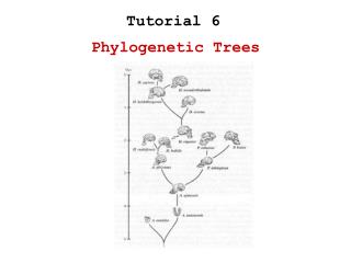
23. Phylogenetic trees • Different ways to represent a phylogenetic tree (illustrated by Treeview)

24. Making a tree from pairwise distances • Distances dij between each pair of sequences iand jare calculated in the given dataset • Different ways defining distances • For nucleotide sequences: Jukes-Cantor, Kimura-2-parameter K2P, HKY (Hasegawa-Kishino-Yano), F84, Tamura-Nei, General time-reversible model, General 12-parameter model • For amino acid sequences: PAM-matrices, BLOSUM-matrices

25. Distance matrix methods • UPGMA • Algorithm introduced by Sokal and Michener 1958 • Neighbor-Joining • Algorithm introduced by Saitou and Nei 1987 • Modified by Studier and Keppler 1988

26. Clustering method: UPGMA • UPGMA = Unweighted pair group method using arithmetic averages • Simple method • It works by clustering the sequences, at each stage connecting two clusters and finally creating a new node on a tree • Method assumes equal rate of evolutionary change along branches  Molecular clock assumption

27. UPGMA A C B • UPGMA produces a rooted tree • Branch lengths satisfy a molecular clock  The divergence of sequences is assumed to occur at the same constant rate at all points in the tree • Trees that are clocklike are rooted and the total branch length from the root up to any leaf is equal • Trees are often referred to be ultrametric • A distance measures are ultrametric if either all three distances are equal dij = dik = djkor two of them are equal and one is smaller: djk < dij = dik  UPGMA is guaranteed to build the correct tree if distances are ultrametric • Method can be used for reconstructing phylogenies if evolutionary rates are assumed to be same in all lineages  criticism in the phylogeny literature • Suitable for the species closely related • Running time O(n2) D

28. Algorithm: UPGMA Initialisation: Assign each sequence i in dataset to its own cluster Define one leaf of T for each sequence, and place at height zero Iteration: Find the two clusters i and j for which dijis the smallest (pick randomly if several equal distances) Define a new cluster ijby Cij = CiU Cj. Cluster ijhas nij = ni + nj members ( initially ni = 1 ) Connect iand jon the tree to a new node v The branch lengths from new node to i and j are placed at height

29. Algorithm: UPGMA (cont.) Iteration (cont.) Compute the distances between the new cluster and the remaining clusters by using Add ij to the current clusters and remove iand j Termination: When only two clusters iandjremain, place the root at height

30. A A B B dAB / 2 C d(AB)C / 2 A B B dAB C dAC dBC UPGMA -- Unweighted Pair Group Method with Arithmetic mean simplest method - uses sequential clustering algorithm (assumption of rate constancy among lineages - often violated) step 1 step 2 (AB) C d(AB)C Distance matrix Tree d(AB)C = (dAC + dAB) / 2

31. UPGMA -- Ilustrations

32. An example UPGMA (1) • Distance matrix (arbitrary) for four items (sequences) A, B, C and D Actually distances are not ultrametric, because three distances are not equal dij≠ dik ≠ djkor two of them are not equal and one is smaller: djk < dij ≠ dik Step 1. Find the smallest distance, dij, between two clusters  A and C, where dij is 7

33. An example UPGMA (2) Step 2. Define new cluster ij, which has nij = ni + nj members (initially ni = 1) New cluster  A and C nAC = nA+ nC=2 Step 3. Connect A and C on the tree to a new node v1 Step 4. The branch lengths from new node v1 to A and C 3,5 A C 3,5

34. An example UPGMA (3) Step 5. Compute the distances between the new cluster AC and the remaining clusters (B and D):

35. An example UPGMA (4) Step 6. Delete the columns and rows of the distance matrix that correspond to clusters A and C, and add a column and a row for cluster AC New distance matrix

36. An example UPGMA (5) • 2nd iteration process • Step 1. Find the two sequences i and j for which dij • is the smallest (randomly if several equal distances) • AC-B • Step 2. Define new cluster (ij), which has nij = ni + nj • members ( initially ni = 1 ) New cluster  AC and B • nACB = nAC+ nB = 2 + 1 = 3 • Step 3. Connect AC and B on the tree to a new node v2 • Step 4. The branch lengths from new node v2 to AC and B •  3.5 A C 3.5 B 4.25

37. An example UPGMA (6) Step 5. Compute the distances between the new cluster and the remaining cluster (D) Step 6. Delete the columns and rows of the distance matrix that correspond to clusters AC and B, and add a column and a row for cluster ACB New distancematrix

38. An example UPGMA (7) Termination: Only two clusters (ACB and D) remaining Place the root height Original distance matrix and final phylogenetic tree(including the branch lengths) 3.5 A 0.75 C 1.92 3.5 B 4.25 D 6.17

39. When UPGMA fails …

40. When UPGMA fails … • The closest leaves are not neighboring leaves; they do not have a common parent node • A test of whether reconstruction is likely to be correct is the ultrametric condition • A distance measures are ultrametric if either all three distances are equal dij = dik = djkor two of them are equal and one is smaller: djk < dij = dik

41. Ultrametric Distances Given three leaves, two distances are equal while a third is smaller: d(i,j)  d(i,k) = d(j,k) a+a  a+b = a+b i nodes i and j are at same evolutionary distance from k – the dendrogram will therefore have ‘aligned’ leaves; i.e. they are all at the same distance from root a b k a j

42. Evolutionary clock speeds Uniform clock: Ultrametric distances lead to identical distances from root to leaves Non-uniform evolutionary clock: leaves have different distances to the root -- an important property is that of additive trees. These are trees where the distance between any pair of leaves is the sum of the lengths of edges connecting them. Such trees obey the so-called 4-point condition (next slide).

43. Additivity • Given a tree, its edge lengths are said to be additive if the distance between any pair of leaves is the sum of the lengths of the edges on the path connecting them • This property is built in automatically as the UMGMA tree is constructed • It is possible for the molecular clock property to fail but for additivity to hold, and in that case there are algorithms that can be used to reconstruct the tree correctly

44. Neighbor Joining • Very popular method • Does not make molecular clock assumption : modified distance matrix constructed to adjust for differences in evolution rate of each taxon • Produces unrooted tree • Assumes additivity: distance between pairs of leaves = sum of lengths of edges connecting them • Like UPGMA, constructs tree by sequentially joining subtrees

45. Neighbor Joining: Once we know the correct (i,j) pair

46. dim=dik+dkm • djm=djk+dkm • dim+djm=dik+djk+2dkm=dij+2dkm • dkm=(dim+djm-dij)/2

47. Neighbour Joining: why not pick the smallest (i,j) pair?

48. j i Neighbour Joining(3)

49. Neighbour Joining: Algorithm

50. Neighbor-Joining: Complexity • The method performs a search using time O(n2) and using time O(n2) to update distance matrix. • Giving a total time complexity of O(n3),and a space complexity of O(n2).