Download
1 / 22
240 likes | 396 Views
Multistage Spectrum Sensing for Cognitive Radios. UCLA CORES. Outline. Introduction Problem Statement Proposal Markov Chain Model Results. Introduction to Spectrum Sensing. Spectral Vacancy. Spectral Vacancy. Spectral Vacancy. The Frequency Spectrum is mostly allocated

E N D
Outline • Introduction • Problem Statement • Proposal • Markov Chain Model • Results
Introduction to Spectrum Sensing Spectral Vacancy Spectral Vacancy Spectral Vacancy • The Frequency Spectrum is mostly allocated • Spectral vacancies exist in: • Unallocated frequency bands. • Allocated bands where the Primary Users (PUs) are spatially absent or temporarily idle. • Cognitive radios (CRs) find spectral vacancies by performing spectrum sensing. • Spectrum Sensing Design Objectives • Maximize the CR throughput • Minimize delay in vacating channel for an incoming PU • Minimize collisions between CRs and PUs PSD Frequency
OSI Model of Cognitive Radios Application Cognitive Radio MAC MAC PHY RF PHY RF . . . Collaborative Sensing Bandwidth Sensing Method Channel • Design Parameters: • Narrowband • Wideband • Design Parameters: • Sensing Algorithm • Sensing Time PU Traffic
Problem Statement No Misdetection (MD) • Conventional Single Stage Sensing • No PU • PU arrives CR Active Sensing CR Active Sensing CR Active Sensing MD -Collision with PU- -Delay in detecting PU- 0 Time 2T T 3T S S S -Throughput Waste- CR Stops Transmission False Alarm (FA) CR Active Sensing No FA PU CR Stops Transmission CR Active Sensing
Multistage Sensing • No PU • PU arrives • Degrees of freedom: • Number of Sensing Stages (S) • Sensing Methods • Sensing Times No MD No MD No MD CR Stops Transmission CR Stops Transmission S1 S2 SS FA FA FA CR Active Sensing Stage 1 CR Active Sensing Stage 1 CR Active Sensing Stage 2 CR Active Sensing Stage S CR Active Sensing Stage 2 CR Active Sensing Stage S MD MD MD No FA No FA No FA PU S1 S2 SS
Previous Work • 802.22 features 2-stage sensing: Coarse and Fine sensing. • Jeon et al* propose a multistage sensing algorithm * W. S. Jeon, D. G. Jeong, J. A. Han, G. Ko, and M. S. Song, "An efficient quiet period management scheme for cognitive radio systems," IEEE Trans. Wireless Comm., vol. 7, no. 2, Feb. 2008. • Limited model; single channel, single sensing algorithm, no collaboration, simple traffic model. • Literature lacks a unified analytical framework that includes Multistage Sensing
Proposal • We introduce a unified analytical framework that models: • Multistage Sensing • Number of sensing stages • Sensing Methods • Algorithm • Sensing Time • Bandwidth • Narrowband • Wideband • CR traffic models • CBR – VBR • Buffered – Unbuffered • Goal is to analyze the impact of varying parameters on: • CR throughput • Delay in vacating channel for a PU • CRs and PUs collisions
Discrete Time Markov Chain • Analysis is based on Markov Chain: • Well established Math tool for modeling discrete space stochastic processes • Future evolution of process depends solely on current state. • Provides closed form/numerical solutions for steady state probabilities and process variables
Assumptions • PUs and CRs arrive and depart at discrete times that are multiples of T • CRs communicating together are synchronized through a control channel • Time taken to switch between communicating and sensing modes is negligible
Model Overview • Model is divided into 3 levels: • CR traffic level • Multistage sensing level • Spectrum Sensing level
ImplementationLevel 1 – CR Traffic Level • PCR ≡ Probability of arrival of a CR • QCR ≡ Probability of departure of a CR • PCR and QCR are tuned to accommodate for different traffic models: • CBR – VBR • Buffered – Unbuffered • (Buffer Size) 1 - PCR 1 - QCR QCR CR Idle CR Sensing and/or Transmitting PCR
ImplementationLevel 2 - Multistage Sensing Level ImplementationLevel 1 – CR Traffic Level CR Sensing and/or Transmitting • S ≡ Number of Sensing Stages 1 - PCR 1 - QCR PU misdetected or no False Alarm QCR CR Sensing and/or Transmitting CR Idle PU detected or False Alarm CR Active Stage 1 CR Active Stage 2 CR Active Stage i CR Active Stage S CR Quiet PCR PU detected or False Alarm
ImplementationLevel 3 – Spectrum Sensing Level ImplementationLevel 2 - Multistage Sensing Level (1-PPU).(1-Pi) CR Active Stage i • PPU ≡ Prob of arrival of a PU • QPU ≡ Prob of departure of a PU • Pi ≡ Prob of False Alarm at Stage i • Qi ≡ Prob of Misdetection at Stage i • PPU and QPU reflect the PU traffic model • Pi and Qi are tuned to describe the sensing method CR Active Stage 1 PU Absent CR Active Stage i PU Absent CR Active Stage i + 1 PU Absent (1-PPU).Pi PPU.(1-Qi) CR Active Stage 1 PU Present CR Active Stage I PU Present CR Active Stage i + 1 PU Present QPU.Pi CR Active Stage i CR Active Stage 1 CR Active Stage 2 CR Active Stage S CR Quiet (1-QPU).(1-Qi) (1-QPU).Qi
Implementation – BandwidthNarrowband Sensing, N Channels 1. 2. CR Idle CR Idle Multistage Sensing Multistage Sensing CR Quiet
Implementation – BandwidthNarrowband Sensing, N Channels Implementation 1: Implementation 2: Ch 1 MSS Ch 1 MSS Ch 1 Quiet CR Active Sensing Stage 1 CR Active Sensing Stage 1 CR Active Sensing Stage 1 CR Active Sensing Stage 1 CR Active Sensing Stage 1 CR Idle Sens. /Tx CR Idle Sens. /Tx CR Quiet CR Quiet Ch 2 MSS Ch 2 MSS Ch 2 Quiet • Example: Single stage, 3 channels: • Example: Single stage, 3 channels: Frequency Frequency Ch N MSS Ch N MSS Ch N Quiet Time Time
Throughput for the Narrowband Case Simulation Configuration
Delay in finding PU Simulation Configuration
Implementation – BandwidthWideband Sensing 1-P 1-P P Frequency IDLE Tx CR Active Sensing Stage 1 CR Active Sensing Stage 3 CR Quiet CR Quiet P CR Active Sensing Stage 2 CR Active Sensing Stage 3 CR Active Sensing Stage 1 CR Idle CR Active Sensing Stage 1 CR Active Sensing Stage 4 CR Active Sensing Stage 1 CR Active Sensing Stage 1 N Channels • Example: Single stage, 3 channels: Time
Throughput for the Wideband Case Simulation Configuration
Simulation Configuration • AWGN independent channels. • Sensing time = , where i is the stage number, L0 = 50 us, Ts = 20 ms, and δ = 2. • Sensing time for the last sensing stage = Ts. • Energy Detection parameters: • Pr = -104 dBm. • Noise Floor = -163 dBm. • BW = 6 MHz • SNR = -8.8 dB. • Energy Threshold = -94.74 dBm. • # of Sensing Nodes = 5. • SU Arrival Probability = 0.2. • SU Departure Probability = 0.2. • PU Arrival Probability = 0.05. • PU Departure Probability = 0.05. • Switching time = 0.2xTs. • 2 Channels • 1000 stages. • 10,000 cycles. Back