Download

1 / 31
310 likes | 408 Views
The tentative schedule of lectures for the semester with links to posted electronic versions of my notes can be found at:. http://crop.unl.edu/claes/PHYS926Lectures.html. Introduction to Elementary Particles , David Griffiths, Harper & Row (1987). The Fundamental Particles

E N D
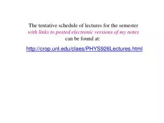
The tentative schedule of lectures for the semester with links to posted electronic versions of my notes can be found at: http://crop.unl.edu/claes/PHYS926Lectures.html
Introduction to Elementary Particles, David Griffiths, Harper & Row (1987). The Fundamental Particles and Their Interactions, 1st Edition, William B. Rolnick Introduction to High Energy Physics, Donald Perkins, Addison-Wesley Publishing.
Two waves of slightly different wavelength and frequency produce beats. x 2 1 k k = x NOTE: The spatial distribution depends on the particular frequencies involved
Many waves of slightly different wavelength can produce “wave packets.”
Adding together many frequencies that are bunched closely together …better yet… integrating over a range of frequencies forms a tightly defined, concentrated “wave packet” A staccato blast from a whistle cannot be formed by a single pure frequency but a composite of many frequencies close to the average (note) you recognize You can try building wave packets at http://phys.educ.ksu.edu/vqm/html/wpe.html
The broader the spectrum of frequencies (or wave number) …the shorter the wave packet! The narrower the spectrum of frequencies (or wave number) …the longer the wave packet!
Fourier Transforms Generalization of ordinary “Fourier expansion” or “Fourier series” Note how this pairs “canonically conjugate” variables and t. Whose product must bedimensionless(otherwisee-itmakesno sense!)
Conjugate variables t, time & frequency: What about coordinate position & ???? inverse distance?? rorx wave number, In fact through the deBroglie relation, you can write:
For a well-localized particle (i.e., one with a precisely known position at x = x0) we could write: Dirac -function a near discontinuous spike at x=x0, (essentially zero everywhere except x=x0) with 1 x x x0 x0 such that f(x)≈ f(x0), ≈constant over x-x, x+x
For a well-localized particle (i.e., one with a precisely known position at x = x0) we could write: In Quantum Mechanics we learn that the spatial wave function(x)can be complemented by the momentum spectrum of the state, found through the Fourier transform: Here that’s Notice that the probability of measuring any single momentum value, p, is: What’s THAT mean? The probability is CONSTANT – equal for ALL momenta! All momenta equally likely! The isolated, perfectly localized single packet must be comprised of an infinite range of momenta!
Remember: (k) (x) k0 (x) (k) k0 …and, recall, even the most general whether confined by some potential OR free actually has some spatial spread within some range of boundaries!
Fourier transforms do allow an explicit “closed” analytic form for the Dirac delta function
Let’s assume a wave packet tailored to be something like a Gaussian (or “Normal”) distribution Area within 1 68.26% 1.28 80.00% 1.64 90.00% 1.96 95.00% 2 95.44% 2.58 99.00% 3 99.46% 4 99.99% A single “damped” pulse bounded tightly within a few of its mean postion, μ. +2 -2 -1 +1
For well-behaved (continuous) functions (bounded at infiinity) likef(x)=e-x2/22 Starting from: -i k g'(x) g(x)= e+ikx f(x) we can integrate this “by parts” f(x) is bounded oscillates in the complex plane over-all amplitude is damped at ±
And so, specifically for a normal distribution:f(x)=e-x2/22 differentiating: from the relation just derived: Let’s Fourier transform THIS statement i.e., apply: on both sides! 1 2 ~ ~ ~ F'(k)e-ikxdk 1 2 ~ ei(k-k)xdx ~ (k – k)
1 2 ~ ei(k-k)xdx ~ (k – k) ~ selecting out k=k k k ' ' rewriting as: dk' dk' ' 0 0
Fourier transforms of one another Gaussian distribution about the origin Now, since: we expect: Both are of the form of a Gaussian! x k 1/
x k 1 or giving physical interpretation to the new variable x px h
xk ~ 2 xp ~ h t ~ 2 tE ~ h
E c B To be charged: means the particle is capable of emitting and absorbing photons e e What’s the ground state or zero-point energy of a system? harmonic oscillator: ½h
The virtual photons in the sea that surround every charged particle, are wavepackets centered at the origin (source of charge) xp ~ h tE ~ h If these describe/map out the electrostatic potential and relate available momentum to be transferred to the distance from the field’s source consider the extremes: other charges may be exposed to the full spectrum of possible momenta x 0 x only vanishingly small momentum transfers are possible
1896 1899 a, b g 1912
Henri Becquerel(1852-1908) received the 1903 Nobel Prize in Physics for the discovery of natural radioactivity. Wrapped photographic plate showed clear silhouettes, when developed, of the uranium salt samples stored atop it. • 1896 While studying the photographic images of various fluorescent & phosphorescent • materials, Becquerel finds potassium-uranyl sulfate spontaneously emits radiation • capable of penetrating thick opaque black paper • aluminum plates • copper plates • Exhibited by all known compounds of uranium (phosphorescent or not) • and metallic uranium itself.
1898Marie Curie discovers thorium (90Th) Together Pierre and Marie Curie discover polonium (84Po) and radium (88Ra) 1899Ernest Rutherfordidentifies 2 distinct kinds of rays emitted by uranium - highly ionizing, but completely absorbed by 0.006 cmaluminum foil or a few cm of air - less ionizing, but penetrate many meters of air or up to a cm of aluminum. 1900P. Villard finds in addition to rays, radium emits - the least ionizing, but capable of penetrating many cm of lead, several feet of concrete
a g B-field points into page b 1900-01 Studying the deflection of these rays in magnetic fields, Becquerel and the Curies establish rays to be charged particles
1900-01 Using the procedure developed by J.J. Thomson in 1887 Becquerel determined the ratio of charge q to mass m for : q/m = 1.76×10¹¹ coulombs/kilogram identical to the electron! : q/m = 4.8×10⁷ coulombs/kilogram 4000 times smaller!
Noting helium gas often found trapped in samples of radioactive minerals, Rutherford speculated that particles might be doubly ionized Helium atoms (He++) 1906-1909Rutherford and T.D.Royds develop their “alpha mousetrap” to collect alpha particles and show this yields a gas with the spectral emission lines of helium! Discharge Tube Thin-walled (0.01 mm) glass tube to vacuum pump & Mercury supply Radium or Radon gas Mercury
Status of particle physics early 20th century Electron J.J.Thomson 1898 nucleus ( proton) Ernest Rutherford 1908-09 a Henri Becquerel 1896 Ernest Rutherford 1899 b g P. Villard 1900 X-rays Wilhelm Roentgen 1895