Chapter 9: Data Retrieval in Sensor Networks
Chapter 9: Data Retrieval in Sensor Networks. Table of Contents. Introduction. Unmanned Aerial/ Ground Vehicle OR Low Flying Airplane. Query. Tank. Introduction. What is a Sensor Network?. BS or Sink (far away). Query from BS to Sensors. Event.

Chapter 9: Data Retrieval in Sensor Networks
E N D
Presentation Transcript
Chapter 9: Data Retrieval in Sensor Networks Table of Contents
Introduction Unmanned Aerial/ Ground Vehicle OR Low Flying Airplane Query Tank
What is a Sensor Network? BS or Sink (far away) Query from BS to Sensors Event
Application of Wireless Sensor Networks in Defense Applications Data Collection Center (BS or Sink) Path between SNs Path of the Query The Path of the Response Query Response
Introduction • A typical Sensor Node (SN) of the network contains several transducers to measure many different physical parameters and any one could be selected under the program control at a given time • The sensed values need to be routed by each SN to the BS either directly or via its CH in a multihop fashion due to power limitations • In a WSN, the overall objective can be defined by the BS and this process is usually known as injection of the query by the BS • In real-life, a low-flying airplane, an unmanned aerial or ground vehicle or a powerful laptop can act as a BS or a sink and usually have adequate source of power • This enables the BS to transmit a query message at a very high power level so as to reach all SNs in a given area simultaneously Such broadcasting is to enable all SNs to start working on the request and the query could also include information about some necessary characteristics of the query
Introduction • If the BS has limited power to reach just few close-by SNs, then the query need to be forwarded/broadcasted to a given area of interest or possibly to the whole WSN • The multi-hop routes are to be employed just like the response is forwarded in a multi-hop fashion • The use of a particular type of query might depend on the application requirements • Sometime, the query may ask for multiple parameters such as temperature, pressure, humidity, etc., and may be required to sense and transmit the values only once, or over a period of time, or use past history to gain statistical information • Based on these, the query can be divided into three categories: • One time queries • Persistent queries • Historical queries
Classifications of WSNs • WSNs can be classified on the basis of their mode of operation or functionality, and the type of target applications • Accordingly, we classify WSNs into three types: • Proactive Networks – The nodes in this network periodically switch on their sensors and transmitters, sense the environment and transmit the data of interest and they provide a snapshot of the relevant parameters at regular intervals and are well suited for applications requiring periodic data monitoring • Reactive Networks – In this scheme, the nodes react immediately to sudden and drastic changes in the value of a sensed attribute and as such, these are well suited for time critical applications • Hybrid Networks – This is a combination of both proactive and reactive networks where sensor nodes not only send data periodically, but also respond to sudden changes in attribute values
Architecture of Sensor Networks The typical hardware platform of a wireless sensor node will consist of: • A simple embedded microcontrollers, such as the Atmel or the Texas Instruments MSP 430 • Currently used radio transceivers include the RFM TR1001 or Infineon or Chipcon devices • Typically, ASK or FSK is used, while the Berkeley PicoNodes employ OOK modulation • Radio concepts like ultra-wideband are in an advanced stage • Batteries provide the required energy as an important concern is battery management and whether and how energy scavenging can be done to recharge batteries in the field • The operating system and the run-time environment is a hotly debated issue in the literature • On one hand, minimal memory footprint and execution overhead are required while on the other, flexible means of combining protocol building blocks are necessary, as meta information has to be used in many places in a protocol stack
Network Architecture • WSN architecture need to cover a desired area both for sensing coverage and communication connectivity point of view • Therefore, density of the WSN network is critical for the effective use of the WSN • There is no well-defined measure of life-time of a WSN and some assume either the failure of a single sensor running out of battery power as life-time of the network • Perhaps a better definition is if certain percentage of sensors stops working, may define the life-time as the network continues to operate • The percentage failure may depend on the nature of application and as long as the area is adequately covered by the operating sensors, a WSN may be considered operational • The SNs are yet to become inexpensive to be deploying with some degree of redundancy
Network Architecture • There is an optimal distance between two sensors that would maximize the sensor lifetime • So, if the density of sensors is high, then some of the sensors can be put into sleep mode to have close to optimal distance between the sensors • Very little work has been done on protocols that suits well to the needs of WSNs • With respect to the radio transmission, the main question is how to transmit as energy efficiently as possible, taking into account all related costs (possible retransmissions, overhead, and so on)
MAC Layer • The MAC and the routing layers are the most active research areas in WSNs • There are two types of schemes available to allocate a single broadcast channel among competing nodes: Static Channel Allocation and Dynamic Channel Allocation • Static Channel Allocation: In this category of protocols, if there are N SNs, the bandwidth is divided into N equal portions in frequency (FDMA), in time (TDMA), in code (CDMA), in space (SDMA) or in schemes such as OFDM or ultra-wideband and since each SN is assigned a private portion, there is no or minimal interference amongst multiple SNs • Dynamic Channel Allocation: In this category of protocols, there is no fixed assignment of bandwidth • When the number of active SNs changes dynamically and data becomes bursty at arbitrary SNs, it is most advisable to use dynamic channel allocation scheme • These are contention-based schemes, where SNs contend for the channel when they have data while minimizing collisions with other SNs’ transmissions
MAC Protocols • WSNs are designed to operate for long time as it is rather impractical to replenish the batteries • However, nodes are in idle state for most time when no sensing occurs • Measurements have shown that a typical radio consumes the similar level of energy in idle mode as in receiving mode • Therefore, it is important that nodes are able to operate in low duty cycles The Sensor-MAC • The Sensor-MAC (S-MAC) protocol explores design trade-offs for energy-conservation in the MAC layer • It reduces the radio energy consumption from the following sources: collision, control overhead, overhearing unnecessary traffic, and idle listening • The basic scheme of S-MAC is to put all SNs into a low-duty-cycle mode –listen and sleep periodically • When SNs are listening, they follow a contention rule to access the medium, which is similar to the IEEE 802.11 DCF
Sensor-MAC • In S-MAC, SNs exchange and coordinate on their sleep schedules rather than randomly sleep on their own • Before each SN starts the periodic sleep, it needs to choose a schedule and broadcast it to its neighbors • To prevent long-term clock drift, each SN periodically broadcasts its schedule as the SYNC packet • To reduce control overhead and simplify broadcasting, S-MAC encourages neighboring SNs to choose the same schedule, but it is not a requirement • A SN first listens for a fixed amount of time, which is at least the period for sending a SYNC packet • If it receives a SYNC packet from any neighbor, it will follow that schedule by setting its own schedule to be the same • Otherwise, the SN will choose an independent schedule after the initial listening period
for SYNC for RTS for CTS Sensor-MAC Listen Sleep Listen Sleep Time • Figure depicts the low-duty-cycle operation of each SN • The listen interval is divided into two parts for both SYNC and data packets • There is a contention window for randomized carrier sense time before sending each SYNC or data (RTS or broadcast) packet
SMACS • The SMACS is an infrastructure-building protocol that forms a flat topology (as opposed to a cluster hierarchy) for sensor networks • SMACS is a distributed protocol which enables a collection of SNs to discover their neighbors and establish transmission/reception schedules for communicating with them without the need for any local or global master nodes • In order to achieve this ease of formation, SMACS combines the neighbor discovery and channel assignment phases • SMACS assigns a channel to a link immediately after the link’s existence is discovered • This way, links begin to form concurrently throughout the network • By the time all nodes hear all their neighbors, they would have formed a connected network • In a connected network, there exists at least one multihop path between any two distinct nodes
SMACS • Since only partial information about radio connectivity in the vicinity of a SN is used to assign time intervals to links, there is a potential for time collisions with slots assigned to adjacent links whose existence is not known at the time of channel assignment • To reduce the likelihood of collisions, each link is required to operate on a different frequency • This frequency band is chosen at random from a large pool of possible choices when the links are formed • This idea is described in Figure 9.6(a) for the topology of Figure 9.5 • Here, nodes A and D wake up at times Ta and Td • After they find each other, they agree to transmit and receive during a pair of fixed time slots • This transmission/reception pattern is repeated periodically every Tframe • Nodes B and C, in turn, wake up later at times Tb and Tc, respectively
Node Discovery Phase in SMACS (b) Node discovery phase
SMACS • The method by which SNs find each other and the scheme by which time slots and operating frequencies are determined constitute an important part of SMACS • To illustrate this scheme, consider nodes B, C, and D shown in Figure 9.6(b) • These nodes are engaged in the process of finding neighbors and wake up at random times • Upon waking up, each node listens to the channel on a fixed frequency band for some random time duration • A node decides to transmit an invitation by the end of this initial listening time if it has not heard any invitations from other nodes • This is what happens to node C, which broadcasts an invitation or TYPE1 message • Nodes B and D hear this TYPE1 message and broadcasts a response, or TYPE2, message addressed to node C during a random time following reception of TYPE1
EAR (Eaves-drop-And-Register) • Mobility can be introduced into a WSN as extensions to the stationary sensor network • Mobile connections are very useful to a WSN and can arise in many scenarios where either energy or bandwidth is a major concern • Where there is the constraint of limited power consumption, small, low bit rate data packets can be exchanged to relay data to and from the network whenever necessary • At the same time, it cannot be assumed that each mobile node is aware of the global network state and/or node positions • Similarly, a mobile node may not be able to complete its task (data collection, network instruction, information extraction) while remaining motionless • Thus, the EAR protocol attempts to offer continuous service to these mobile nodes under both mobile and stationary constraints • EAR is a low-power protocol that allows for operations to continue within the stationary network while intervening at desired moments for information exchange
EAR • The EAR algorithm employs the following four primary messages: • Broadcast Invite (BI) – This is used by the stationary node to invite other nodes to join and if multiple BIs are received, the mobile node continues to register every stationary node encountered, until its registry becomes full • Mobile Invite (MI) – This message is sent by the mobile node in response to the BI message from the stationary node for establishing connection • Mobile Response (MR) – This is sent by the stationary node in response to a MI message, and indicates the acceptance of the MI request which causes the stationary node to select slots along the TDMA frame for communication and the stationary node will enter the mobile node in its own registry • Mobile Disconnect (MD) – With this message, the mobile node informs the stationary node of a disconnection and for energy saving purposes, no response is needed from the stationary node
The STEM • The Sparse Topology and Energy Management (STEM) protocol is based on the assumption that most of the time the sensor network is only sensing the environment, waiting for an event to happen • In other words, STEM may be seen as better suitable for reactive sensor networks where the network is in the monitoring state for vast majority of time • One example of such an application is a sensor network designed to detect fires in a forest • These networks have to remain operational for months or years, but sensing only on the occurrence of a forest fire • Clearly, although it is desirable that the transfer state be energy-efficient, it may be more important that the monitoring state be ultra-low-power as the network resides in this state for most of the time • This observation holds true for many other applications as well
The STEM • The idea behind STEM is to turn on only a node’s sensors and some preprocessing circuitry during monitoring states • Whenever a possible event is detected, the main processor is woken up to analyze the sensed data in detail and forward it to the data sink • However, the radio of the next hop in the path to the data sink is still turned off, if it did not detect the same event • STEM solves this problem by having each node to periodically turn on its radio for a short time to listen if someone else wants to communicate with it • The node that wants to communicate, i.e. , the initiator SN, sends out a beacon with the ID of the node it is trying to wake up, i.e. , the target SN • This can be viewed as a procedure by which the initiator SN attempts to activate the link between itself and the target SN • As soon as the target SN receives this beacon, it responds back to the initiator node and both keep their radio on at this point
The STEM • If the packet needs to be relayed further, the target SN will become the initiator node for the next hop and the process is repeated • Once both the nodes that make up a link have their radio on, the link is active and can be used for subsequent packets • However, the actual data transmissions may still interfere with the wakeup protocol • To overcome this problem, STEM proposes the wakeup protocol and the data transfer to employ different frequency bands as depicted in Figure 9.7 • In addition, separate radios would be needed in each of these bands • In Figure 9.7 we see that the wakeup messages are transmitted by the radio operating in frequency band f1 • STEM refers to these communications as occurring in the wakeup plane • Once the initiator SN has successfully notified the target SN, both SNs turn on their radio that operates in frequency band f2 • The actual data packets are transmitted in this band, called the data plane
The Stem Wakeup plane = f1 Data plane = f2
Routing Layer • Routing in sensor networks is usually multi-hop • The goal is to send the data from source node(s) to a known destination node • The destination node or the sink node is known and addressed by means of its location • A BS may be fixed or mobile, and is capable of connecting the sensor network to an existing infrastructure where the user can have access to the collected data • The task of finding and maintaining routes in WSNs is nontrivial since energy restrictions and sudden changes in node status (e.g., failure) cause frequent unpredictable topological changes • Thus, the main objective of routing techniques is to minimize the energy consumption in order to prolong WSN lifetime • To achieve this objective, routing protocols proposed in the literature employ some well-known routing techniques as well as tactics special to WSNs • To preserve energy, strategies like data aggregation and in-network processing, clustering, different node role assignment, and data-centric methods are employed
Routing Layer • In sensor networks, conservation of energy is considered relatively more important than quality of data sent • Therefore, energy-aware routing protocols need to satisfy this requirement • Routing protocols for WSNs have been extensively studied in the last few years • Routing protocols for WSNs can be broadly classified into flat-based, hierarchical-based, and adaptive, depending on the network structure • In flat-based routing, all nodes are assigned equal role • In hierarchical-based routing, however, nodes play different roles and certain nodes, called cluster heads (CHs), are given more responsibility • In adaptive routing, certain system parameters are controlled in order to adapt to the current network conditions and available energy levels • Furthermore, these protocols can be classified into multipath-based, query-based, negotiation-based, or location-based routing techniques
Network Structure Based • In this class of routing protocols, the network structure is one of the determinant factors • In addition, the network structure can be further subdivided into flat, hierarchical and adaptive depending upon its organization Flat Routing • In flat routing based protocols, all nodes play the same role and we present the most prominent protocols falling in this category Directed Diffusion • Directed Diffusion is a data aggregation and dissemination paradigm for sensor networks • It is a data-centric (DC) and application-aware approach in the sense that all data generated by sensor nodes is named by attribute-value pairs • Directed Diffusion is very useful for applications requiring dissemination and processing of queries • The main idea of the DC paradigm is to combine the data coming from different sources en-route (in-network aggregation) by eliminating redundancy, minimizing the number of transmissions; thus saving network energy and prolonging its lifetime
Data Centric Routing and Directed Diffusion • Unlike traditional end-to-end routing, DC routing finds routes from multiple sources to a single destination (BS) that allows in-network consolidation of redundant data • In Directed Diffusion, sensors measure events and create gradients of information in their respective neighborhoods • The BS requests data by broadcasting interests, which describes a task to be done by the network • Interest diffuses through the network hop-by-hop, and is broadcast by each node to its neighbors • As the interest is propagated throughout the network, gradients are setup to draw data satisfying the query towards the requesting node • Each SN that receives the interest setup a gradient toward the SNs from which it receives the interest • This process continues until gradients are setup from the sources back to the BS
Data Centric Routing and Directed Diffusion • The strength of the gradient may be different towards different neighbors, resulting in variable amounts of information flow • At this point, loops are not checked, but are removed at a later stage • Figure 9.9 depicts an example of the operation of directed diffusion • Figure 9.9(a) presents the propagation of interests, Figure 9.9(b) shows the gradients construction, and Figure 9.9(c) depicts the data dissemination • When interests fit gradients, paths of information flow are formed from multiple paths, and the best paths are reinforced so as to prevent further flooding according to a local rule • In order to reduce communication costs, data is aggregated on the way The BS periodically refreshes and re-sends the interest when it starts to receive data from the source(s) • This retransmission of interests is needed because the medium is inherently unreliable
Data Centric Routing and Directed Diffusion • Sensor nodes in a directed diffusion-based network are application-aware, which enables diffusion to achieve energy savings by choosing empirically good paths and by caching and processing data in the network • An application of directed diffusion is to spontaneously propagate an important event to regions of the sensor network • Such type of information retrieval is well suited for persistent queries where requesting nodes expect data that satisfy a query for a period of time
Data Centric Routing and Directed Diffusion • The performance of data aggregation methods employed by the directed diffusion paradigm is affected by the location of the source nodes in the network, the number of sources, and the network topology • In order to investigate these factors, two models of source placement shown in Figure 9.10 have been investigated • These models are called the event radius (ER) model, and the random sources (RS) model • In the ER model, a single point in the network area is defined as the location of an event • For example, this may correspond to a vehicle or some other phenomenon being tracked by the sensor nodes • All nodes within a distance S (called the sensing range) of this event that are not sinks, are considered to be data sources • In the RS model, K nodes that are not sinks are randomly selected to be sources • Unlike the ER model, in the RS model the sources are not necessarily close to each other
Network Structure Based Event Radius (ER) model Randum source (RS) model
Sequential Assignment Routing (SAR) • The routing scheme in SAR depends on three factors: energy resources, QoS on each path, and the priority level of each packet • To avoid single route failure, a multi-path approach coupled with a localized path restoration scheme is employed • To create multiple paths from a source node, a tree rooted at the source node to the destination nodes (i.e. , the set of BSs) is constructed • The paths of the tree are defined by avoiding nodes with low energy or QoS guarantees • At the end of this process, each sensor node is a part of multi-path tree • For each SN, two metrics are associated with each path: delay (which is an additive QoS metric); and energy usage for routing on that path • The energy is measured with respect to how many packets will traverse that path • SAR calculates a weighted QoS metric as the product of the additive QoS metric and a weight coefficient associated with the priority level of the packet • The goal of SAR is to minimize the average weighted QoS metric for the network
Minimum Cost Forwarding Algorithm • The minimum cost forwarding algorithm (MCFA) exploits the fact that the direction of routing is always known, that is, towards fixed and predetermined external BS • Therefore, a SN need not have a unique ID nor maintain a routing table • Instead, each node maintains the least cost estimate from itself to the BS • Each message forwarded by the SN is broadcast to its neighbors • When a node receives the message, it checks if it is on the least cost path between the source SN and the BS • If so, it re-broadcasts the message to its neighbors • This process repeats until the BS is reached • In MCFA, each sensor node should know the least cost path estimate from itself to the BS
Coherent and Non-Coherent Processing • Data processing is a major component in the operation of any WSN • In general, sensor nodes cooperate with each other in processing different data flooded throughout the network • Two examples of data processing techniques are coherent and non-coherent data processing-based routing • In non-coherent data processing routing, nodes locally process the raw data before being sent to other nodes for further processing • The nodes that perform further processing are called the aggregators • In coherent routing, the data is forwarded to aggregators after minimum processing of time stamping and duplicate suppression • To perform energy-efficient routing, normally coherent processing is selected
Energy Aware Routing • This protocol is similar to directed diffusion (discussed earlier) with the difference that it maintains a set of paths instead of maintaining or enforcing one optimal path • These paths are maintained and chosen by means of a certain probability, which depends on how low the energy can be conseved for each path • By selecting different routes at different times, the energy of any single route will not deplete so quickly • The protocol initiates a connection through localized flooding, which is used to discover all routes between source/destination pair and their costs; thus building up the routing tables • Next, the high-cost paths are discarded and a forwarding table is constructed by choosing neighboring nodes inversely proportional to their cost • Then, data is sent to the destination using the forwarding table with a probability that is inversely proportional to the node cost • Finally, to keep the various paths alive, localized flooding is carried out by the destination node
Hierarchical Routing • Hierarchical, or cluster-based routing has its roots in wired networks, where the main goals are to achieve scalable and efficient communication • As such, the concept of hierarchical routing has also been employed in WSN to perform energy-efficient routing • In a hierarchical architecture, higher energy nodes (usually called cluster heads) can be used to process and send the accumulated information while low energy nodes can be used to sense in the neighborhood of the target and pass on to the CH • In these cluster-based architectures creation of clusters and appropriate assignment of special tasks to CHs can contribute to overall system scalability, lifetime, and energy efficiency • An example of a general hierarchical clustering scheme is depicted in Figure 9.11 • As we can see from this figure, each cluster has a CH which collects data from its cluster members, aggregates it and sends it to the BS or an upper level CH
Hierarchical Routing or sink
Cluster Based Routing Protocol (CBRP) • A simple cluster based routing protocol (CBRP) divides the network nodes into a number of overlapping or disjoint two-hop-diameter clusters in a distributed manner • The cluster members just send the data to the CH, and the CH is responsible for routing the data to the destination • The major drawback with CBRP is that it requires a lot of hello messages to form and maintain the clusters, and thus may not be suitable for WSN • Given that sensor nodes are stationary in most of the applications this is a considerable and unnecessary overhead Scalable Coordination • In hierarchical clustering method, the cluster formation appears to require considerable amount of energy as periodic advertisements are needed to form the hierarchy • Also, any changes in the network conditions or sensor energy level result in re-clustering which may be not quite acceptable as some parameters tend to change dynamically
Low-Energy Adaptive Clustering Hierarchy Low-Energy Adaptive Clustering Hierarchy (LEACH) • LEACH is a hierarchical clustering algorithm for sensor networks, called Low-Energy Adaptive Clustering Hierarchy (LEACH) • LEACH is a good approximation of a proactive network protocol, with some minor differences which includes a distributed cluster formation algorithm • LEACH randomly selects a few sensor nodes as CHs and rotates this role amongst the cluster members so as to evenly distribute the energy dissipation across the cluster • In LEACH, the CH nodes compress data arriving from nodes that belong to the respective cluster, and send an aggregated packet to the BS in order to reduce the amount of information that must be transmitted • LEACH uses a TDMA and CDMA MAC to reduce intra-cluster and inter-cluster collisions, respectively, while data collection is centralized and is performed periodically
Power-Efficient Gathering in Sensor Information Systems (PEGASIS) • The Power-Efficient Gathering in Sensor Information Systems (PEGASIS) is a near optimal chain-based protocol which is an enhancement over LEACH • In order to prolong network lifetime, nodes employing PEGASIS communicate with their closest neighbors only and they take turns in communicating with the BS • Whenever a round of nodes communicating with the BS ends, a new round starts • This decreases the power required to transmit data per round, as energy dissipation is spread uniformly over all nodes and as a result, PEGASIS has two main goals • First, it aims at increasing the lifetime of each node by using collaborative techniques, as a result, the overall network lifetime is also increased • Second, it only allows coordination between nodes that are close together, thus reducing the bandwidth consumed for communication • To locate the closest neighbor SN, SNs use the signal strength to measure the distance to all of its neighboring nodes and then adjust the signal strength so that only one node can be heard
Small Minimum Energy Communication Network (MECN) • The minimum energy communication network (MECN) protocol has been designed to compute an energy-efficient subnetwork for a given sensor network • On top of MECN, a new algorithm called Small MECN (SMECN) has been proposed to construct such a subnetwork • The subnetwork (i.e. , subgraph G') constructed by SMECN is smaller than the one constructed by MECN if the broadcast region around the broadcasting node is circular for a given power assignment • The subgraph G' of graph G, which represents the sensor network, minimizes the energy consumption satisfying the following conditions: • The number of edges in G' is less than in G, while containing all nodes in G • The energy required to transmit data from a node to all its neighbors in subgraph G' is less than the energy required to transmit to all its neighbors in graph G • The resulting subnetwork computed by SMECN helps in the task of sending messages on minimum-energy paths
Threshold-sensitive Energy Efficient (TEEN) Threshold-sensitive Energy Efficient (TEEN) • A Threshold-sensitive Energy Efficient sensor Network (TEEN) protocol has been depicted in Figure 9.12 • In this scheme, at every cluster change time, the CH broadcasts the following to its members in addition to the attributes: • Hard Threshold (HT): This is a threshold value for the sensed attribute • It is the absolute value of the attribute beyond which, the node sensing this value must switch on its transmitter and report to its CH • Soft Threshold (ST): This is a small change in the value of the sensed attribute which triggers the node to switch on its transmitter and transmit once the HT has been crossed • In TEEN, nodes sense their environment continuously, thereby making it appropriate for real time applications
Features Suited for time critical sensing applications Time critical data reaches the user almost instantaneously At every cluster change time, the parameters are broadcast afresh and so, the user can change them as required Energy consumption can be controlled by changing the threshold values Attribute > Threshold Cluster Formation Clutser-Head Reveives Message Cluster Change Time Threshold-sensitive Energy Efficient (TEEN) Parameters
Features It offers flexibility by allowing the user to set the threshold values for the attributes Attributes can be changed every cluster change Drawback If threshold HT not reached then user never gets to know about the network Application Time critical environment like intrusion detection, etc. TEEN Reactive Protocol
APTEEN (Adaptive Periodic Threshold Sensitive Energy Efficient Sensor Network Protocol) Combines features of Reactive and Proactive Networks Periodicity and threshold values controlled by the user Energy Efficient Protocol Hybrid Protocol (UC)
To take advantage of both the networks, it is preferable to have both the features in the system (UC) Functioning [Attributes, Thresholds (HT ,ST), Count Time (TC)] are broadcast to all cluster members Parameters Attributes > Threshold CLUSTER FORMATION Cluster-Head Receives Message Cluster Change Time Periodic Intervals Hybrid Protocol (APTEEN)