Download

1 / 31
370 likes | 601 Views
Chapter 11 Phylogenetic Tree Construction Methods and Programs. Character based methods Molecular sequences from individual taxa Characters at corresponding positions in alignments are homologous Characters of common ancestor can be traced Each character evolved independently

E N D
Chapter 11 Phylogenetic Tree Construction Methods and Programs
Character based methods • Molecular sequences from individual taxa • Characters at corresponding positions in alignments are homologous • Characters of common ancestor can be traced • Each character evolved independently • Distance based methods • Dissimilarity between sequence pairs, based on alignment • All sequences involved are homologous • Tree branches are additive
Distance methods: Clustering-based methods • Unweighted Pair Group Method Using Arithmetic Average (UPGMA) • Given distance matrix • Group two taxa with smallest pairwise distance • Generate new matrix with combined taxa as a single group • Repeat grouping and reduce matrix again • Continue iteration until all taxa are grouped • Last taxon added considered outgroup and tree root
Distance methods: Clustering-based methods Neighbour Joining Similar to UPGMA, but does not assume constant evolutionary rate between taxa Makes use of distance matrix, but corrects for unequal evolutionary rates by calculating r-distances and transformed r-distances d’AB = dAB -1/2(rA+rB) d’AB is the converted distance between A and B and dAB is the actual evolutionary distance between A and B rA (or rB) is sum of distances of A (or B) to all other taxa ri = dij Where i and j are two different taxa r value is needed to create a modified distance matrix Transformed r: r’i = ri/(n-2) Used to determine distance of individual taxon to nearest node
Generalized neighbour joining • Disadvantage of NJ is that one tree is generated • Depending on choice of two equally close starting taxa, sub-optimal tree may be calculated • Generalized NJ: multiple NJ runs with different starting taxa • Select tree from all calculated trees that best fit actual evolutionary distances
Optimally based methods: Fitch-Margoliash • Selects best tree based on minimal deviation between calculated distance and original distance • Randomly selects two taxa, and calculated branch lengths • Examines all tree topologies and chooses one with minimum deviation • dij pairwise distance • pij corresponding tree branch length E =
Minimum evolution (ME) Similar to FM, but uses different optimality criterion to find tree with minimum branch length S = bi bi is ith branch length ME slightly outperforms FM
Character based Methods : Maximum Parsimony (thriftiness) Based on character differences in sequence alignments Number of differences counted, i.e., ancestral sequences can be inferred Tree with fewest evolutionary changes (Occam’s Razor) Occam’s Razor (14th-century English logician and Franciscan friar, William of Ockham.) "entia non sunt multiplicanda praeter necessitatem", roughly translated as "entities must not be multiplied beyond necessity“, i.e., "All other things being equal, the simplest solution is the best."
William of Ockham - Sketch labelled "frater Occham iste", from a manuscript of Ockham's Summa Logicae, 1341
Maximum Parsimony • Search all possible tree topologies • Reconstruct ancestral tree that require minimum number of character changes • Use only sites with rich phylogenetic information to save time • Informative sites: two different kinds of characters occurring at least twice
Weighted parsimony • Weighing scheme takes into account functionally important sites • Transitions versus transversion
Tree searching methods • Only works for < 10 taxa • Need simplification steps for more taxa: branch and bound
Branch and Bound • Upper limit for number of allowed sequence variations • Build tree for all taxa involved using UPGMA or NJ • Compute minimum substitutions for such a tree • MP must be equal or better than UPGMA or NJ
When number of taxa > 20 • Branch and bound computationally too intensive • Need heuristic approach • Cut of branch and re-graft • Recalculate branch lengths • Continue iteration until no shorter branch arrangements are found • Can get stuck in “local minima” • Global sub-pruning option in some programs
Long Branch Attraction • Rapidly evolving taxa with long branches are places together in a tree • Assumption that all taxa evolve at the same rate • All mutations (transitions and transversions) contribute equally to branch lengths • Weighted parsimony should solve problem • Increase taxon sampling size
Maximum likelihood method • The probability that a nucleotide changes over time t is calculated from • Pt = 1/4 + 1/4e-t • The probabilities are multiplied from root to tip for all branches • All possible tree topologies are examined, and probabilities calculated • The tree with the highest probability is chosen
Quartet Puzzling • Make many subsets composed of four taxa • Combine all “quartets” into single tree • Significantly reduces computing time • ML tree not guaranteed
Neighbour Joining Maximum Likelihood • Construct initial tree with NJ • “Poor” branches (low bootstrap support), collapsed • Resolve by ML • 10X faster than neat ML method
Genetic Algorithm • Generate random population of trees with arbitrary branch lengths • Select tree with highest likelihood score • Allow this tree to “mutate:” • Screen “mutated offspring”, and select highest likelihood trees • Repeat process until no higher scoring trees are produced
Bayesian Analysis Based on posterior probability Probably the fastest and most accurate phylogenetic analysis available to date Posterior probability =
Phylogenetic Tree Evaluation • Bootstrapping • Recalculate trees with randomly perturbed datasets • If the original tree topology is repeatedly found, it is most likely correct • Parametric • New datasets are generated based on sequence distribution • Based opn sequence substitution model (Jukes-Cantor or Kimura) • Non-parametric bootstrapping • Random replacement of sites • Jack knifing • Randomly delete half of the sites in a dataset
Bayesian simulation • Most efficient in terms of statistical evaluation • Does not require bootstrapping because MCMC procedure millions of re-sampling steps • Posterior probabilities assigned as statistical support • Makes statistical valuation of ML trees more feasible
Kishino-Hasegawa Test • Test whether two competing tree topologies are statistically significantly different • Difference in branch length at each informative site is calculated • Standard deviation of the difference values is them calculated • Allowing derivation of t-value
Shimodaira-Hasegawa Test Frequently used for ML Based on 2 test Converted to p-value
Phylogenetic Programs PAUP* http://paup.csit.fsu.edu/ Phylip http://evolution.genetics.washington.edu/phylip.html TREE-PUZZLE http://www.tree-puzzle.de PHYML http://atgc.lirmm.fr/phyml/ MrBayes http://morphbank.ebc.uu.se/mrbayes