Download
1 / 8
80 likes | 175 Views
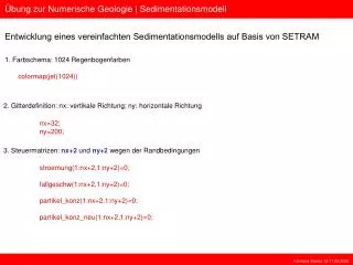
Übung zur Numerische Geologie | Sedimentationsmodell. Entwicklung eines vereinfachten Sedimentationsmodells auf Basis von SETRAM . 1. Farbschema: 1024 Regenbogenfarben colormap(jet(1024)). 2. Gitterdefinition: nx: vertikale Richtung; ny: horizontale Richtung. nx=32; ny=200;.

E N D
Übung zur Numerische Geologie | Sedimentationsmodell Entwicklung eines vereinfachten Sedimentationsmodells auf Basis von SETRAM 1. Farbschema: 1024 Regenbogenfarben colormap(jet(1024)) 2. Gitterdefinition: nx: vertikale Richtung; ny: horizontale Richtung nx=32; ny=200; 3. Steuermatrizen: nx+2 und ny+2 wegen der Randbedingungen stroemung(1:nx+2,1:ny+2)=0; fallgeschw(1:nx+2,1:ny+2)=0; partikel_konz(1:nx+2,1:ny+2)=0; partikel_konz_neu(1:nx+2,1:ny+2)=0; Klemens Seelos 13-17.05.2005
Übung zur Numerische Geologie | Sedimentationsmodell 4. Strömungsdefinition stroemung(1:16,1:ny+2)= 7.5; stroemung(16:32,1:ny+2)= 3.5; 5. Definition der Fallgeschwindigkeit (nach Stokes); ~ 6 cm/s entspricht einem runden 300 µm Quarzkorn fallgeschw(1:nx+2,1:ny+2)=2; 6. Definition der Partikelkonzentration partikel_konz(2,4)=.2; Klemens Seelos 13-17.05.2005
Übung zur Numerische Geologie | Sedimentationsmodell 7. Definition der Schleifenwiederholungen (Iterationen), ohne Abbruchkriterium! z=1; zmax=250; 8. Definition des Modellkerns (gekoppelte while- und for-Schleifen) while z <= zmax for i=2:nx for j=2:ny … partikel_konz_neu(i,j) = (fallgeschw(i-1,j) x partikel_konz(i-1,j) + stroemung(i,j-1) x partikel_konz(i,j-1))/ (fallgeschw(i+1,j) + stroemung(i,j+1)) end end z = z+1; end Fortsetzung mit der Grafikausgabe innerhalb der Schleife Klemens Seelos 13-17.05.2005
Übung zur Numerische Geologie | Sedimentationsmodell 9. Definition der Grafikausgabe if rem(z,5) == 0 pause(.1) surf(interp2(partikel_konz_neu(:,:),2),'EdgeColor','none') view(2); caxis([0 .05]) box on set(gcf,'Color',[.95 .95 .98]) set(gca,'XTick',[ ],'YTick',[ ]) set(gca,'YDir','reverse') title('Partikeltransport [Upstream-Schema 1.Ordnung]','color',[.6 .2 .2],'FontSize',7) set(gca,'XColor',[.6 .6 .8],'YColor',[.6 .6 .8]) set(gca,'FontSize',7,'Color','w') set(gca,'PlotBoxAspectRatio',[ny+2,nx+2,1]) set(gca,'Color',[.95 .95 .98]) colorbar('horiz') set(colorbar('horiz'),'FontSize',7) end Klemens Seelos 13-17.05.2005
Übung zur Numerische Geologie | Sedimentationsmodell 9. Neudefinition der Startzelle (dient zur Gewährleistung des Sedimentnachschubs) partikel_konz_neu(2,4,1)=.2; partikel_konz = partikel_konz_neu; 10. Schließen der äußeren while-Schleife z = z+1; end Klemens Seelos 13-17.05.2005
Übung zur Numerische Geologie | Sedimentationsmodell Multi-Korngrößen-Modell clear all % stroemung: horizontaler Strömungsanteil % fallgeschw: vertikaler Strömungsanteil (Fallgeschwindigkeit abhängig von der Partikelgrösse/-dichte) % residuum: reale Partikelkonzentration pro Zelle % partikel_konz: finites partikel_konz (mit den Koordinaten nx, ny) stroemung=[ ]; partikel_konz=[ ]; fallgeschw=[ ]; % Gitterdefinition: nx: vertikale Richtung; ny: horizontale Richtung nx=32; ny=200; % Strömungsmatrix: nx+2 wegen Randbedingungen stroemung(1:nx+2,1:ny+2)=0; Klemens Seelos 13-17.05.2005
Übung zur Numerische Geologie | Sedimentationsmodell konz_ebenen=3; fallgeschw(1:nx+2,1:ny+2,1:konz_ebenen)=0; partikel_konz(1:nx+2,1:ny+2,1:konz_ebenen)=0; % Definition von unterschiedlichen Strömungen im Kanal (vertikal geschichtet) stroemung(1:8,1:ny+2)= 7.5; stroemung(8:32,1:ny+2)= 3; stroemung(22:32,1:ny+2)= -2; % Definition der unterschiedlichen Partikelgrößen (konz_ebenen) fallgeschw(1:nx+2,1:ny+2,1)=6; % 300µm Partikel fällt 6 cm/s fallgeschw(1:nx+2,1:ny+2,2)=3; % 220µm Partikel fällt 3 cm/s fallgeschw(1:nx+2,1:ny+2,3)=1.25; % 120µm Partikel fällt 0.9 cm/s % Vorgabe der Partikelkonzentration in der primären Zelle partikel_konz(2,4,1:konz_ebenen)=.2; Klemens Seelos 13-17.05.2005
Übung zur Numerische Geologie | Sedimentationsmodell % Iterationen z=1; zmax=150; % Modellkern: Berechnungsschleife while z<=zmax k=1; while k<=konz_ebenen for i=2:nx for j=2:ny if stroemung(i,j)<0 partikel_konz(2,4,k)=.2; partikel_konz(i,j,k)=(fallgeschw(i-1,j,k)*partikel_konz(i-1,j,k)+abs(stroemung(i,j+1))*partikel_konz(i,j+1,k))/... (fallgeschw(i+1,j,k)+abs(stroemung(i,j-1))); elseif stroemung(i,j)>0 partikel_konz(2,4,k)=.2; partikel_konz(i,j,k)=(fallgeschw(i-1,j,k)*partikel_konz(i-1,j,k)+stroemung(i,j-1)*partikel_konz(i,j-1,k))/... (fallgeschw(i+1,j,k)+stroemung(i,j+1)); end end end k=k+1; end z=z+1 end Klemens Seelos 13-17.05.2005