Problem Solving and Optimization Strategies in Lecture 2
Explore problem solving strategies, search techniques, and optimization methods in computer science. Learn about uninformed and informed search, A* algorithm, simulated annealing, and genetic algorithms.

Problem Solving and Optimization Strategies in Lecture 2
E N D
Presentation Transcript
Lecture 2 – Problem Solving, Search and Optimization Shuaiqiang Wang (王帅强) School of Computer Science and Technology Shandong University of Finance and Economics http://www2.sdufe.edu.cn/wangsq/ shqiang.wang@gmail.com
What are Problems Here? • Property • Nondeterministic • Partially observable • State: A representation of current information • Solution: A plan or a policy • An feasible/optimal state • A feasible/optimal sequence of states • Search!
Q ( ) ((1,1))
Q Q ( ) ((1,1)) ((1,1) (2,3))
Q ( ) ((1,1)) ((1,1) (2,3))
Q Q ( ) ((1,1)) ((1,1) (2,3)) ((1,1) (2,4))
Q Q ( ) Q ((1,1)) ((1,1) (2,3)) ((1,1) (2,4)) ((1,1) (2,4) (3.2))
Q Q ( ) ((1,1)) ((1,1) (2,3)) ((1,1) (2,4)) ((1,1) (2,4) (3.2))
Q ( ) ((1,1)) ((1,1) (2,3)) ((1,1) (2,4)) ((1,1) (2,4) (3.2))
( ) ((1,1)) ((1,1) (2,3)) ((1,1) (2,4)) ((1,1) (2,4) (3.2))
Q ( ) ((1,1)) ((1,2)) ((1,1) (2,3)) ((1,1) (2,4)) ((1,1) (2,4) (3.2))
Q Q ( ) ((1,1)) ((1,2)) ((1,1) (2,3)) ((1,1) (2,4)) ((1,2) (2,4)) ((1,1) (2,4) (3.2))
Q Q ( ) Q ((1,1)) ((1,2)) ((1,1) (2,3)) ((1,1) (2,4)) ((1,2) (2,4)) ((1,1) (2,4) (3.2)) ((1,2) (2,4) (3,1))
Q Q ( ) Q ((1,1)) ((1,2)) Q ((1,1) (2,3)) ((1,1) (2,4)) ((1,2) (2,4)) ((1,1) (2,4) (3.2)) ((1,2) (2,4) (3,1)) ((1,2) (2,4) (3,1) (4,3))
Search Strategies • Search strategies are evaluated along the following dimensions: • Completeness: does it always find a solution if one exists? • Time complexity: number of nodes generated • Space complexity: maximum number of nodes in memory • Optimality: does it always find a least-cost solution?
Categories • Uninformed search • Breadth-first search • Depth-first search • Informed search • A* search • Hill-climbing search • Simulated annealing search • Genetic algorithms
A* Search • Idea: avoid expanding paths that are already expensive • Evaluation function f(n) = g(n) + h(n) • g(n) = cost so far to reach n • h(n) = estimated cost from n to goal • f(n) = estimated total cost of path through n to goal
Algorithm • Add the starting square (or node) to the open list. • Repeat the following:a) Look for the lowest F cost square on the open list. We refer to this as the current square.b) Switch it to the closed list.c) For each of the 8 squares adjacent to this current square … • If it is not walkable or if it is on the closed list, ignore it. Otherwise do the following. • If it isn't on the open list, add it to the open list. Make the current square the parent of this square. Record the F, G, and H costs of the square. • If it is on the open list already, check to see if this path to that square is better, using G cost as the measure. A lower G cost means that this is a better path. If so, change the parent of the square to the current square, and recalculate the G and F scores of the square. If you are keeping your open list sorted by F score, you may need to resort the list to account for the change. • d) Stop when you: • Add the target square to the closed list, in which case the path has been found (see note below), or • Fail to find the target square, and the open list is empty. In this case, there is no path.
Hill-Climbing Problem: depending on initial state, can get stuck in local maxima
Simulated Annealing • Idea: escape local maxima by allowing some "bad" moves but gradually decrease their frequency
Genetic Algorithm • A genetic representation of potential solutions to the problem. • A way to create a population (an initial set of potential solutions). • An evaluation function rating solutions in terms of their fitness. • Genetic operators that alter the genetic composition of offspring (selection, crossover,mutation, etc.). • Parameter values that genetic algorithm uses (population size, probabilities of applying genetic operators, etc.). In general, a GA has 5 basic components
General Structure crossover encoding CC(t) Initial solutions t 0P(t) offspring start chromosome mutation CM(t) offspring selection N new population termination condition? decoding P(t) + C(t) solutions candidates Y roulette wheel stop fitness computation best solution evaluation
Heuristic Search = Optimization Evaluation function f(n) Objective function f(x) Search Optimization Solution
Optimization • Definition: • Local search • Hill-Climbing • Simulated Annealing • Genetic Algorithms
Conventional Optimization • Based on derivation/gradient • Construct F(x) based on f, g and h, and let • For example: • Problem: For many problems, F(x) is very complicated, and it is very difficult to solve the differential equations