Download

1 / 15
150 likes | 191 Views
Learn about Kuhn-Tucker optimality criteria, differentiation between interior and exterior solutions, KKT conditions, and optimizing constrained problems.

E N D
Optimality Criteria • Big question: How do we know that we have found the “optimum” for min f(x)? • Answer: Test the solution for the “necessary and sufficient conditions”
Optimality Conditions – Unconstrained Case • Let x* be the point that we think is the minimum for f(x) • Necessary condition (for optimality): f(x*) = 0 • A point that satisfies the necessary condition is a stationary point • It can be a minimum, maximum, or saddle point • How do we know that we have a minimum? • Answer: Sufficiency Condition: The sufficient conditions for x* to be a strict local minimum are: f(x*) = 0 2f(x*) is positive definite
Constrained Case – KKT Conditions • To proof a claim of optimality in constrained minimization (or maximization), we have to check the found point with respect to the (Karesh) Kuhn Tucker conditions. • Kuhn and Tucker extended the Lagrangian theory to include the general classical single-objective nonlinear programming problem: minimize f(x) Subject to gj(x) 0 for j = 1, 2, ..., J hk(x) = 0 for k = 1, 2, ..., K x = (x1, x2, ..., xN)
Interior versus Exterior Solutions • Interior: If no constraints are active and (thus) the solution lies at the interior of the feasible space, then the necessary condition for optimality is same as for unconstrained case: f(x*) = 0 • Exterior: If solution lies at the exterior, then the condition f(x*) = 0 does not apply because some constraints will block movement to this minimum. • Some constraints will (thus) be active. • We cannot get any more improvement (in this case) if for x* there does not exist a vector d that is both a descent direction and a feasible direction. • In other words: the possible feasible directions do not intersect the possible descent directions at all. • See Figure 5.2
Mathematical Form • A vector d that is both descending and feasible cannot exist if -f = mi (gi) (with mi 0) for all active constraints iI. • See page 152-153 • This can be rewritten as 0 = f + mi (gi) • This condition is correct IF feasibility is defined as g(x) 0. • If feasibility is defined as g(x) 0, then this becomes -f = mi (-gi) • Again, this only applies for the active constraints. • Usually the inactive constraints are included as well, but the condition mj gj = 0 (with mj 0) is added for all inactive constraints jJ. • This is referred to as the complimentary slackness condition. • Note that this condition is equivalent to stating that mj= 0 for inactive constraints • Note that I+J = m, the total number of (inequality) constraints.
Necessary KKT Conditions For the problem: Min f(x) s.t. g(x) 0 (n variables, m constraints) The necessary conditions are: f(x) + migi(x) = 0 (optimality) gi(x) 0 for i = 1, 2, ..., m (feasibility) mi gi(x) = 0 for i = 1, 2, ..., m (complementary slackness condition) mi 0 for i = 1, 2, ..., m (non-negativity) Note that the first condition gives n equations.
Necessary KKT Conditions (General Case) • For general case (n variables, M Inequalities, L equalities): Min f(x) s.t. gi(x) 0 for i = 1, 2, ..., M hj(x) = 0 for J = 1, 2, ..., L • In all this, the assumption is that gj(x*) for j belonging to active constraints and hk(x*) for k = 1, ...,K are linearly independent • This is referred to as “constraint qualification” • The necessary conditions are: f(x) + migi(x) + ljhj(x) = 0 (optimality) gi(x) 0 for i = 1, 2, ..., M (feasibility) hj(x) = 0 for j = 1, 2, ..., L (feasibility) mi gi(x) = 0 for i = 1, 2, ..., M (complementary slackness condition) mi 0 for i = 1, 2, ..., M (non-negativity) (Note: lj is unrestricted in sign)
Necessary KKT Conditions (if g(x)0) • If the definition of feasibility changes, the optimality and feasibility conditions change. • The necessary conditions become: f(x) - migi(x) + ljhj(x) = 0 (optimality) gi(x) 0 for i = 1, 2, ..., M (feasibility) hj(x) = 0 for j = 1, 2, ..., L (feasibility) mi gi(x) = 0 for i = 1, 2, ..., M (complementary slackness condition) mi 0 for i = 1, 2, ..., M (non-negativity)
Restating the Optimization Problem • Kuhn Tucker Optimization Problem: Find vectors x(Nx1), m(1xM) and l(1xK) that satisfy: f(x) + migi(x) + ljhj(x) = 0 (optimality) gi(x) 0 for i = 1, 2, ..., M (feasibility) hj(x) = 0 for j = 1, 2, ..., L (feasibility) mi gi(x) = 0 for i = 1, 2, ..., M (complementary slackness condition) mi 0 for i = 1, 2, ..., M (non-negativity) • If x* is an optimal solution to NLP, then there exists a (m*, l*) such that (x*, m*, l*) solves the Kuhn–Tucker problem. • Above equations not only give the necessary conditions for optimality, but also provide a way of finding the optimal point.
Limitations • Necessity theorem helps identify points that are not optimal. A point is not optimal if it does not satisfy the Kuhn–Tucker conditions. • On the other hand, not all points that satisfy the Kuhn-Tucker conditions are optimal points. • The Kuhn–Tucker sufficiency theorem gives conditions under which a point becomes an optimal solution to a single-objective NLP.
Sufficiency Condition • Sufficient conditions that a point x* is a strict local minimum of the classical single objective NLP problem, where f, gj, and hk are twice differentiable functions are that • The necessary KKT conditions are met. • The Hessian matrix 2L(x*) = 2f(x*) + mi2gi(x*) + lj2hj(x*) is positive definite on a subspace of Rn as defined by the condition: yT2L(x*) y 0 is metfor every vector y(1xN) satisfying: gj(x*)y = 0 for j belonging to I1 ={ j | gj(x*) = 0, uj* > 0} (active constraints) hk(x*)y = 0 for k = 1, ..., K y 0
KKT Sufficiency Theorem (Special Case) • Consider the classical single objective NLP problem. minimize f(x) Subject to gj(x) 0 for j = 1, 2, ..., J hk(x) = 0 for k = 1, 2, ..., K x = (x1, x2, ..., xN) • Let the objective function f(x) be convex, the inequality constraints gj(x) be all convex functions for j = 1, ..., J, and the equality constraints hk(x) for k = 1, ..., K be linear. • If this is true, then the necessary KKT conditions are also sufficient. • Therefore, in this case, if there exists a solution x* that satisfies the KKT necessary conditions, then x* is an optimal solution to the NLP problem. • In fact, it is a global optimum.
Limitations • .
Closing Remarks • Kuhn-Tucker Conditions are an extension of Lagrangian function and method. • They provide powerful means to verify solutions • But there are limitations… • Sufficiency conditions are difficult to verify. • Practical problems do not have required nice properties. • For example, You will have a problems if you do not know the explicit constraint equations (e.g., in FEM). • If you have a multi-objective (lexicographic) formulation, then I would suggest testing each priority level separately.