Download
1 / 46
460 likes | 622 Views
Noura Al-Zoubi Advisor: Dr. Abdalla Obeidat Co-advisor: Dr. Maen Gharaibeh. Nucleation rates of ethanol and methanol using an equation of state. Out Lines :. Introduction.

E N D
Noura Al-Zoubi Advisor: Dr. Abdalla Obeidat Co-advisor: Dr. Maen Gharaibeh Nucleation rates of ethanol and methanol using an equation of state.
Out Lines: • Introduction. • First order phase transition. • Classical nucleation theory (CNT). • Gradient theory (GT). • Computational methodology. • Results and conclusion.
. Definition Nucleation is the process which the formation of new phases begins and is thus a widely spread phenomenon in both nature and technology. Nucleation refers to the kinetic processes involved in the initiation of the first order phase transition in non equilibrium systems. Condensation and evaporation, crystal growth, deposition of thin films and overall crystallization are only a few of the processes in which nucleation plays a prominent role.
First Order Phase Transitions pressure – volume diagram for pure fluid for different isotherms.
dependence of the reduced pressure and Gibbs energy on the reduced volume using VDW
Classical Nucleation TheorySurface and volume energies of formation a cluster versus cluster radius. The energy of formation has a maximum at critical radius.
P-form: -form: S-form: In (CNT) , the work of formation have different forms
Experimental data for methanol illustratingthe inadequate temperature dependence predicted by S-form.
Experimental data for ethanol illustrating the inadequate temperature dependence predicted by S-form.
DFT Advantages Powerful technique that has been used to explore varies systems. Disadvantages Require exact intermolecular Potential. GT Advantages Requires a Cubic EOS Disadvantages An approximation to DFT Density functional theory and the road to gradient theory
Gradient Theory • The Helmholtz free energy density is given as: • The density profile can be determined by integrating the following equation: • The work of formation is given as:
Experimental nucleation rates of methanol compared to the predictionsof GT with the CPHB EOS.
Experimental nucleation rates of ethanol compared to the predictions of GT with the CPHB EOS.
SAFT-EOS • Exact EOS for low T • Cubic EOS
Equilibrium Densities of liquid and vapor 1. Conditions 2. Calculations using Newton-Raphson method do row(1)=guess1 row(2)=guess2 k(1,1)=dp(row(1),t) k(1,2)=-dp(row(2),t) k(2,1)=dmew(row(1),t) k(2,2)=-dmew(row(2),t) f(1)=p(row(2),t)-p(row(1),t) f(2)=mew(row(2),t)-mew(row(1),t) z=k(2,1)/k(1,1) k(2,1)=0.0d0 f(2)=f(2)-(z*f(1)) k(2,2)=k(2,2)-(z*k(1,2)) u(2)=f(2)/k(2,2) u(1)=(f(1)-k(1,2)*u(2))/k(1,1) row=row+u end do Computational Methodology
Influence Parameter • Experimental surface tension Surface=(23.88-0.08807*(T-273))*10-7 • GT surface tension • Equivalence between GT and experimental surface tensions C=(Surface/integral)2 /2 where C: influence parameter Integral= • Calculations using Composite Simpson method step=4001 h1=(row(1)-row(2))/step sum=0.d0 sum1=0.d0 do i=1,(step/2.d0)-1 x1=row(2)+2.d0*i*h1 x2=row(2)+(2.d0*i-1)*h1 sum=sum+(2.d0*h1/3.d0)*deltaW(x1,row(2),t) sum1=sum1+(4.d0*h1/3.d0)*deltaW(x2,row(2),t) end do integral=(h1/3.d0)*(deltaW(row(2),row(2),t)+deltaW(row(1),row(2),t))+ sum+sum1
Droplet Density Profile • Second order differential Equation where • Boundary conditions as and as
Tridiagonal Matrix • Construction of tridiagonal matrix do do i=2,steps Aa(i)=i-2 B1(i)=-1*(i-1)*(2.d0+hv2*dmew(U(i),t)/CValue) Cc(i)=i RR(i)=(i-1)*hv2*Gg(U(i),nb,t)/CValue end do Aa(1)=0 B1(1)=-(6.d0+hv2*dmew(U(1),t)/CValue) Cc(1)=6.d0 Cc(steps)=0 RR(1)=hv2*Gg(U(1),nb,t)/CValue RR(steps)=(steps-1)*hv2*Gg(U(steps),nb,t)/CValue-(steps)*nb
Flat Density Profile • Second order differential equation • First order differentioal Equation • Calculations using Runga-Kutta method x11=(row1+row2)/2.d0 o i=1.d0,500.d0 dx1=((mew(x11,t)-mew(row2,t))/dmew(x11,t)) x11=x11-dx1 if((dabs(dx1))<upsilon) exit end do interval=35.d-8/(step-1), mm=22.d-8/interval, ub(mm)= x11 do i=(22.d-8/interval),1.d0,-1.d0 f11=interval*diff(Ub(i),row2,t), f12=interval*diff(Ub(i)+0.5d0*f11,row2,t) f13=interval*diff(ub(i)+0.5d0*f12,row2,t), f14=interval*diff(ub(i)+f13,row2,t) Ub(i) =Ub(i)+(f11+2.0d0*f12+2.0d0*f13+f14)/6.0d0 , ub(i-1)=ub(i) end do Ub(mm)=x11 do i=(22.d-8/interval),step f11=interval*diff(Ub(i),row2,t), f12=interval*diff(Ub(i)-0.5d0*f11,row2,t) f13=interval*diff(Ub(i)-0.5d0*f12,row2,t), f14=interval*diff(Ub(i)-f13,row2,t) Ub(i)=Ub(i)-(f11+2.0d0*f12+2.0d0*f13+f14)/6.0d0 ub(i+1)=ub(i) end do
Solution of Tridiagonal Matrix • Lower Upper (LU) Decomposition method n=steps bet=b1(1) u(1)=rr(1)/bet do j=2,n gam(j)=cc(j-1)/bet bet=b1(j)-aa(j)*gam(j) u(j)=(rr(j)-aa(j)*u(j-1))/bet end do do j=n-1,1,-1 u(j)=u(j)-gam(j+1)*u(j+1) end do
The S value to start from! do i=1,steps U(i)=(U(i)-rhog)*(nref-nb)/(rhol-rhog)+nb end do do do i=2,steps Aa(i)=i-2 B1(i)=-1*(i-1)*(2.d0+hv2*dmew(U(i),t)/CValue) Cc(i)=i RR(i)=(i-1)*hv2*Gg(U(i),nb,t)/CValue end do Aa(1)=0 B1(1)=-(6.d0+hv2*dmew(U(1),t)/CValue) Cc(1)=6.d0 Cc(steps)=0 RR(1)=hv2*Gg(U(1),nb,t)/CValue RR(steps)=(steps-1)*hv2*Gg(U(steps),nb,t)/CValue-(steps)*nb
Comparison between flat density profile and density profile at S=1.65
Density profiles from S=1.65 to S=6 at T=300K filename1='Density_at_S_1_6_5_0.txt' do l1=1,6 do mm=0,9 do qq=0,8,9 do vv=0,8,9 sa=l1+mm/10.0d0+qq/100.0d0 +vv/1000.0d0 , if(sa<=1.650d0) cycle nb=sa*rhog do i=1,MAX dnb=(p(nb,t)-sa*p(rhog,t))/dp(nb,t), nb=nb-dnb, if((dabs(dnb))<upsilon) exit end do open(13,file=filename1,status="old",action="read",iostat=fstat) do k=1,steps read(13,'(f18.16)') U(k) end do do k=1,steps U(k)=U(k)+nb-nb1 end do 1
do do i=1,steps Aa(i)=i-2 B1(i)=-1.d0*(i-1)*(2.d0+hv2*dmew(U(i),t)/CValue) Cc(i)=i RR(i)=(i-1)*hv2*Gg(U(i),nb,t)/CValue end do Aa(1)=0 B1(1)=-(6.d0+hv2*dmew(U(1),t)/CValue) Cc(1)=6.d0 Cc(steps)=0 RR(1)=hv2*Gg(U(1),nb,t)/CValue RR(steps)=(steps-1)*hv2*Gg(U(steps),nb,t)/CValue-(steps)*nb end do end do end do end do call tridag_ser(aa,b1,cc,RR,X1,steps) error=0.d0 do i=1,steps error=error+(X1(i)-U(i))**2 end do error=sqrt(dabs(error)) U=X1 if (error<Upsilon) exit end do 2
Results for density profiles with different supersaturation values.
filename1='Density_at_S_6_0_0_0.txt' do T=300.d0,230.d0,-1.d0 if(T==300.d0)cycle do row(1)=guess1 row(2)=guess2 k(1,1)=dp(row(1),t) k(1,2)=-dp(row(2),t) k(2,1)=dmew(row(1),t) k(2,2)=-dmew(row(2),t) f(1)=p(row(2),t)-p(row(1),t) f(2)=mew(row(2),t)-mew(row(1),t) z=k(2,1)/k(1,1) k(2,1)=0.0d0 f(2)=f(2)-(z*f(1)) k(2,2)=k(2,2)-(z*k(1,2)) u1(2)=f(2)/k(2,2) u1(1)=(f(1)-k(1,2)*u1(2))/k(1,1) row=row+u1 error1=0.0d0 do i=1,2 error1=error1+f(i)**2 end do error1=dsqrt(error1) if (error1<Upsilon) exit guess1=row(1) guess2=row(2) end do Ts=T-273.15d0 gama = (23.88d0-.08807d0*Ts)*1.d-7 row1=row(1) row2=row(2) steps=4001 h1=(row1-row2)/steps Density profiles from T=300K to T=230K at S=6 1
do k1=1,steps read(13,'(f18.16)') U(k1) end do close(13) do k1=1,steps U(k1)=U(k1)+nb-nb1 end do counter=0 do sum=0.d0 sum1=0.d0 do i=1,(steps/2.d0)-1 x1=row2+2.d0*i*h1 x2=row2+(2.d0*i-1)*h1 sum=sum+(2.d0*h1/3.d0)*deltaW(x1,row2,t) sum1=sum1+(4.d0*h1/3.d0)*deltaW(x2,row2,t) end do integral=(h1/3.d0)*(deltaW(row2,row2,t)+deltaW(row1,row2,t))+sum+sum1 cvalue=(gama/integral)**2/2.d0 rhog=row(2) rhol=row(1) sa=6.d0 nb=sa*rhog do i=1,MAX dnb=(p(nb,t)-sa*p(rhog,t))/dp(nb,t) nb=nb-dnb if((dabs(dnb))<upsilon) exit print*,i,dnb end do hv=(35.d-8/(steps-1)) hv2=hv**2 nb1=nb open(13,file=filename1,status="old",action="read",iostat=fstat read(13,'(I7)') steps counter=counter+1 do i=2,steps Aa(i)=i-2 B1(i)=-1.d0*(i-1)*(2.d0+hv2*dmew(U(i),t)/CValue) Cc(i)=i RR(i)=(i-1)*hv2*Gg(U(i),nb,t)/CValue 2
end do Aa(1)=0 B1(1)=-(6.d0+hv2*dmew(U(1),t)/CValue) Cc(1)=6.d0 Cc(steps)=0.d0 RR(1)=hv2*Gg(U(1),nb,t)/CValue RR(steps)=(steps-1)*hv2*Gg(U(steps),nb,t)/CValue-(steps)*nb call tridag_ser(aa,b1,cc,RR,X11,steps) errors=0.d0 do i=1,steps error=error+(X11(i)-U(i))**2 end do error=sqrt(error)/steps U=X1 if (errors<upsilon) exit end do count1=int((T+.1d0)/100.d0) count2=int((T+.1d0-count1*100)/10) count3=int(T+.1d0-count1*100-count2*10) count4=int((T-int(T+.1d-4))*10+.1d-2) count5=int((T-int(T+.1d-4))*100-count4*10+.1d-2) filename2='Density_at_T_'//achar(count1+48)//achar(count2+48)//achar(count3+48)//achar(count4+48)//achar(count5+48)//'.txt' open(12,file=filename2,status="replace",action="write",position="rewind",iostat=gstat) do k1=1,steps write(12,'(f18.16)') U(k1) end do close(12) end do 3
Density profiles from S=6 to S=2 at T=293K T=293.d0 Ts=T-273.15d0 gama = (23.88d0-.08807d0*Ts)*1.d-7 cvalue=5.974465658636744d-10 sa=6.d0 rhog=3.656930116927259d-6 rhol=1.711839175934329d-2 nb=sa*rhog do i=1,MAX dnb=(p(nb,t)-sa*p(rhog,t))/dp(nb,t) nb=nb-dnb if((dabs(dnb))<upsilon) exit end do hv=(35.d-8/(steps-1)) hv2=hv**2 nb1=nb filename1='Density_at_T_2_9_3.txt' do sa=6.0d0,2.0d0,-.01d0 ll=int(sa/10.d0) mm=int(sa+.001d0-ll*10.d0) qq=int((sa+.001d0-ll*10.d0-mm)*10.d0) vv=int((sa+.001d0-ll*10.d0-mm-qq/10.d0)*100.d0) nb=sa*rhog do i=1,MAX dnb=(p(nb,t)-sa*p(rhog,t))/dp(nb,t) nb=nb-dnb 1
B1(1)=-(6.d0+hv2*dmew(U(1),t)/CValue) Cc(1)=6.d0 Cc(steps)=0 RR(1)=hv2*Gg(U(1),nb,t)/CValue RR(steps)=(steps-1)*hv2*Gg(U(steps),nb,t)/CValue-(steps)*nb call tridag_ser(aa,b1,cc,RR,X1,steps) error=0.d0 do i=1,steps error=error+(X1(i)-U(i))**2 end do error=sqrt(error) U=X1 if (error<epsilon) exit end do open(13,file=filename2,status="replace",action="write",position="rewind",iostat=gstat) do k=1,steps write(13,'(f18.16)') U(k) end do close(13) filename1=filename2 nb1=nb end do if((dabs(dnb))<upsilon) exit end do if(sa<=1.99d0) cycle if(sa>=6.0d0) cycle open(12,file=filename1,status="old",action="read",iostat=fstat) if(fstat==0) print*,trim(filename1),' opened' read(12,'(I7)') steps do k=1,steps read(12,'(f18.16)') U(k) end do close(12) do k=1,steps U(k)=U(k)+nb-nb1 end do counter=0 do counter=counter+1 do i=1,steps Aa(i)=i-2 B1(i)=-1.d0*(i-1)*(2.d0+hv2*dmew(U(i),t)/CValue) Cc(i)=i RR(i)=(i-1)*hv2*Gg(U(i),nb,t)/CValue end do Aa(1)=0 2
Results for density profiles with different supersaturation values at T=293K
Work of formation • Integral Equation • Calculations results1=0.0 do i=4,steps-3 results1=results1+(w0(U(i),nb,t)-w0(nb,nb,t))*hv2*((i1)**2)+ ((cValue*dabs((U(i+1)-U(i-1)))**2)/8.0d0)*((i-1)**2) end do results1=results1+bb*((w0(U(2),nb,t)-w0(nb,nb,t))*hv2*((2-1)**2)+ ((cValue*dabs((U(3)-U(1)))**2)/8.0d0)*((2-1)**2)) results1=results1+cc*((w0(U(3),nb,t)-w0(nb,nb,t))*hv2*((3-1)**2)+ ((cValue*dabs((U(4)-U(2)))**2)/8.0d0)*((3-1)**2)) results1=results1+aa*((w0(U(steps),nb,t)-w0(nb,nb,t))*hv2*((steps-1)**2)+ ((cValue*dabs((nb-U(steps-1)))**2)/8.0d0)*((steps-1)**2)) results1=results1+bb*((w0(U(steps-1),nb,t)-w0(nb,nb,t))*hv2*((steps-2)**2)+ ((cValue*dabs((U(steps)-U(steps-2)))**2)/8.0d0)*((steps-2)**2)) results1=results1+cc*((w0(U(steps-2),nb,t)-w0(nb,nb,t))*hv2*((steps-3)**2))+ ((cValue*dabs((U(steps-1)-U(steps-3)))**2)/8.0d0)*((steps-3)**2)) GW1=4.d0*Pi*hv*results1/(kb*T)
Nucleation Rate • Equation Where • Calculation GJ1=dsqrt(2.d4*gama/(PI*ma))*(sa*P(rhol,t)/(kb*T))**2/rhom*1.d0*dexp(-GW1)
Comparison of the experimental rates(open circles) for methanol with two versions of CNT and GT based on the SAFT EOS.
Comparison of the experimental rates (open circles) for ethanol with two versions of CNT, and GT based on the SAFT EOS.
Number of molecules in critical nucleus • Integral Equation • Calculations hw=35.d0/(steps-1) results3=0.0 do i=4,steps-3 results3=results3+(U(i)-nb)*(i-1)**2*hw**2 end do results3=results3+bb*(U(2)-nb)*(2-1)**2*hw**2 results3=results3+cc*(U(3)-nb)*(3-1)**2*hw**2 results3=results3+aa*(U(steps)-nb)*(steps-1)**2*hw**2 results3=results3+cc*(U(steps-1)-nb)*(steps-2)**2*hw**2 results3=results3+bb*(U(steps-2)-nb)*(steps-3)**2*hw**2 ngt=4*pi*results3*hw
Conclusions: • GT improved temperature dependence of nucleation rates for both ethanol and methanol. • GT improved supersaturation dependence of nucleation rates exactly for methanol, but for ethanol, GT couldn’t improve the supersaturation dependence of nucleation rates.