Download
1 / 42
430 likes | 763 Views
Theory and practice of X-ray diffraction experiment. Power Point presentation from lecture # 2 is available at: http://dl.dropbox.com/u/23622306/UIUC/Lecture%202.ppt. Power Point presentation from lecture # 4 is available at: http://dl.dropbox.com/u/23622306/UIUC/lecture%204.ppt.

E N D
Theory and practice of X-ray diffraction experiment Power Point presentation from lecture # 2 is available at: http://dl.dropbox.com/u/23622306/UIUC/Lecture%202.ppt Power Point presentation from lecture # 4 is available at: http://dl.dropbox.com/u/23622306/UIUC/lecture%204.ppt
Grain size and types of diffraction experiment • Single crystal • Bulk powder • Nanopowder • Amorphous/glass
z hkl X-ray x Reciprocal space • Direct space relates to atoms in the unit cell, while reciprocal space relates to peaks in diffraction experiment. • In diffraction experiment planes of atoms in the crystal act as a “selective” mirror and reflect (in the same way as in optics) incoming beam of x-rays if specific geometric conditions are satisfied. • Vectors in reciprocal space correspond to families of planes in the crystal (the direction of the rec. vector is normal to the family of planes). • In a conventional crystal (as opposed to incommensurately modulated crystal or quasi-crystal) vectors in reciprocal space can occupy only points on a 3-dimensional grid. • Grid coordinates of reciprocal vectors are known as Miller indices hkl • Geometry of the reciprocal space grid is determined by the unit cell of the crystal. And can be directly measured. • D-spacing is equal to inverse of the reciprocal vector length. • Coordinates of vectors in reciprocal space are described in laboratory (instrument-related) reference coordinate system. y
Orientation matrix • UB matrix relates the Miller indices of reciprocal vector (hkl) with its Cartesian coordinates in lab reference system (xyz) at zero goniometer position. xyz=UB hkl • Columns in the orientation matrix are coordinates of the principal vectors in reciprocal space 1 0 0 , 0 1 0 and 0 0 1. • UB matrix is composed of two sub-matrices, U and B • U describes the orientation of the crystal axes with respect to the laboratory reference system, while B stores information about the unit cell parameters. • By inverting the above equation one can calculate what are the Miller indices of a measured reciprocal vector xyz hkl=UB-1 xyz z hkl X-ray x y
hkl Diffraction condition and Bragg equation for a single crystal 1q hkl nl=2dsinq diffracted X-ray 2q incident X-ray 1q 2q Diffraction geometry is analogous to reflection in a selective mirror: Diffraction is effective only at selected incidence angles with respect to the “reflecting” plane, determined by the Bragg equation. When diffraction is effective “reflection” angle equals to the incidence angle, with the reciprocal vector bisecting the two. Intensity of the “reflected” beam is not equal to the intensity of the incident beam, it is related to the mean electron density within the direct lattice plane.
Explanation of Bragg derivation nl=2dsinq
Ewald construction • In diffraction experiment we measure the direction and intensity of the diffracted beams as well as the orientation of the crystal corresponding to each of the diffraction peaks. • Diffraction does not occur at any arbitrary crystal orientation. In general to bring a given reciprocal vector to a diffraction position one may need to rotate the sample using goniometer or change the incident wavelength (an exception is polychromatic experiment in which a range of incident wavelengths is available). • When the diffraction event occurs, the following relation between the incident and diffracted beam vectors, incident wavelength and the reciprocal vector is satisfied: • R is the goniometer rotation matrix bringing the crystal from the zero-goniometer position to the position at which maximum peak intensity is observed. • In the Ewald construction the center of the crystal and the center of reciprocal space do not coincide. 1/l(S0+Sd)=R xyz Rxyz Sd S0 Radius of the Evald sphere is 1/l
Experimental approach to single crystal diffraction Effective diffraction vs. observed diffraction • Cause effective diffraction and find (observe) diffraction signal • Measure Sd and R for a number of diffraction peaks • Calculate xyz using the Ewald equation • Find orientation matrix/index the peaks (assign Miller indices) • Measure/calculate peak intensities I(hkl) Wide oscillation ± 13° Monochromatic SXD experiment
Atomic scattering factor • The incoming X-rays are scattered by the electrons of the atoms. As the wavelength of the X-rays (1.5 to 0.5 A) is of the order of the atom diameter, most of the scattering is in the forward direction. For neutrons of the same wavelength the scattering factor is not angle dependent due to the fact that the atomic nucleus is magnitudes smaller than the electron cloud. It is also obvious that the X-ray scattering power will depend on the number of electrons in the particular atom. The X-ray scattering power of an atom decreases with increasing scattering angle and is higher for heavier atoms. A plot of scattering factor f in units of electrons vs. sin(theta)/lambda shows this behavior. Note that for zero scattering angle the value of f equals the number of electrons. Electron density around an isolated atom (r) is spherically symmetric, with max at nucleus position, and falls off smoothly with distance. Cromer and Mann 9-parameter equation
Anomalous dispersion The scattering factor contains additional (complex) contributions from anomalous dispersion effects (essentially resonance absorption) which become substantial in the vicinity of the X-ray absorption edge of the scattering atom. These anomalous contributions can be calculated as well and their presence can be exploited in the MAD phasing technique.
Excitation Scans We can observe the Δf” by measuring the absorption of the x-rays by the atom. Often we us the fluorescence of the absorbing atom as a measure of absorptivity. That is, we measure an “excitation” spectrum. How to get Δf ’? The real, “dispersive” component is calculated from Δf” by the Kramers-Kronig relationship. Very roughly, Δf’ is the negative first derivative of Δf”. From Ramakrishnan’s study of GH5
Thermal vibrations and Debye-Waller factor • There is an additional weakening of the scattering power of the atoms by the so called Temperature-, B- , or Debye-Waller factor. This exponential factor is also angle dependent and effects the high angle reflections substantially (one of the reasons for cryo-cooling crystals is to reduce the attenuation of the high angle reflections due to this B-factor).
Lorenz correction • Accounts for the different speed with which the reciprocal vectors move through the Ewald sphere
Other intensity corrections • Absorption correction • Extinction correction • Preferred orientation • Illuminated volume • Incident intensity
Symmetry of peak intensities. Friedel pairs and Laue classes • Friedel's law, named after Georges Friedel, is a property of Fourier transforms of real functions.1 • Given a real function , its Fourier transform • has the following properties. • where is the complex conjugate of . • Centrosymmetric points are called Friedel's pairs. • The Friedel pair symmetry is broken by anomalous dispersion. The effect is strongly pronounced for incident energies close to the absorption edge.
Systematic absences and space group determination A centered hkl k + l = 2n B centered h + l = 2n C centered h + k = 2n F centered k + l = 2n, h + l = 2n, h + k = 2n I centered h + k + l = 2n R (obverse) -h + k + l = 3n R (reverse) h - k + l = 3n Glide reflecting in a 0kl b glide k = 2n c glide l = 2n n glide k + l = 2n d glide k + l = 4n Glide reflecting in b h0l a glide h = 2n c glide l = 2n n glide h + l = 2n d glide h + l = 4n Glide reflecting in c hk0 b glide k = 2n a glide h = 2n n glide k + h = 2n d glide k + h = 4n Screw || [100] h00 21, 42 h = 2n 41, 43 h = 4n Screw || [010] 0k0 21, 42 k = 2n 41, 43 k = 4n Screw || [001] 00l 21, 42, 63 l = 2n 31, 32, 62, 64 l = 3n 41, 43 l = 4n 61, 65 l = 6n
Point detector experiment • Scintillator detector converts x-ray to electric signal • Center the sample on rotation axis and with the beam • Search for peaks (usually 10-20) at different 2theta and sample orientations • Center the peaks that were found • Determine orientation matrix • Find more peaks to constrain and refine the orientation matrix better • Calculate position for a list of peaks that need to be measured based on orientation matrix • Position each peak individually, record a rocking curve/peak profile • Integrate, scale and correct peak intensities • Solve/refine the structure
Area detector experiment • CCD detector detects visible light. Phosphor screen in front of the detector converts x-ray to visible light. • Center the sample on rotation axis and with the beam • Collect diffraction images while rotating the sample • Determine detector coordinates and sample orientations for each diffraction peak • Reconstruct the reciprocal space in 3-d and determine the orientation matrix (index) • Predict peak positions in recorded diffraction images and retrieve peak intensities (structure factor amplitudes) • Solve/refine the structure
Area detector and step scan approach With wide rotation image we determine the direction of the diffracted beam Sd but the rotation angles (necessary to calculate R) at which each peak occurs are unknown. Step scan allows to determine R for each peak by finding a step image at which the peak has maximum intensity. With R and Sd we can calculate xyz. Step scan images
zoom fitting Residual General algorithm for analysis of single-crystal XRD data Image Initial peak list (Sd) Step scan analysis (R) Orientation matrix (UB) Predicted peak list Integrated intensities I(hkl) Scaled and corrected intensities
Demonstration of single-crystal data processing with GSE_ADA
Powder diffraction • Sample is composed of a very large (preferably >106)number of single crystal specimens with random distribution of crystal orientations. • Diffraction for all reciprocal vectors occurs (is effective) at any arbitrary orientation of the sample. Sample rotation is not necessary. • Single crystal diffraction peaks (directional beams) become cones of radiation. • Peaks corresponding to different reciprocal vectors (different hkls) that have similar length (d-spacing) overlap. • Diffraction signal carries only information about the length of the reciprocal vectors, but not their orientation.
Different experimental approaches to powder diffraction • Polychromatic EDX approach • White beam • Point energy-dispersive detector at fixed angle • Non-scanning signal accumulation • Can provide access to large d-spacing range w/o much of angular access • Suffers from preferred orientation problems • Peak usually quite broad • Peak intensity interpretation difficult (correction) • Monochromatic approach with point detector • Mono beam • Point detector at variable angle • Scanning signal accumulation • Suffers from preferred orientation problems • Can provide patterns with very narrow peak profiles • Monochromatic approach with area detector • Mono beam • Area detector at fixed or variable angle/position • Non-scanning signal accumulation • Does not suffer from preferred orientation problems
Integration of 2-dimensional diffraction pattern • Calibration of detector geometry • Detector coordinates of the point of intersection of the incident beam and the detector surface • Sample-to-detector distance • Detector non-orthogonality with respect to the beam • Pixel size • Goniometer geometry calibration • Goniometer zeros • Goniometer axis alignment with the detector orientation • Instrumental function • Calibrating with a diffraction standard • Cake transform
Energy dispersive powder diffraction Ge solid state semiconductor detector Multiple wavelengths
Powder pattern fitting techniques • Individual peak fitting • Peak positions are not constrained – they are individually refined • Peak profiles are not related with each other • Closely overlapping peaks are very hard to deal with • LeBail (unit-cell constrained) refinement • Individual peak positions are not refined – they are calculated from the unit cell parameters which are refined • Individual peak profiles are not refined – there is a global function (e.g. Cagliotti function) that connects all peak profiles. • Peak intensities are refined free (not constrained by the structure model) • Gives much more reliable way of refining positions and intensities of closely overlapping peaks. • Rietveld (model-biased) refinement • Individual peak positions are not refined – they are calculated from the unit cell parameters which are refined • Individual peak profiles are not refined – there is a global function (e.g. Cagliotti function) that connects all peak profiles. • Individual peak intensities are not refined free, they are calculated from the structure model which is refined.
Peak width analysis • Instrumental function • Focused beam divergence away from the sample • Detector pixel size • Phosphor point spread function • Sample-related factors • Scherrer formula • Hall-Williamson plot • Cagliotti function • Deconvolution size = K l / FW(S) cos(q) FW(S) cos(q) = K l / size + 4 strain sin(q) FW(S)D = FWHMD - FW(I)D The dimensionless shape factor K has a typical value of about 0.9, but varies with the actual shape of the crystallite. Scherrer formula is not applicable to grains larger than about 0.1 μm, which precludes those observed in most metallographic and ceramographic microstructures.
Peak width analysis 13nm nano powder FW(S) cos(q) = K l / size + 4 strain sin(q) Bulk fine powder
Tools of the tradePowder diffraction • Image integration • Fit2d • Powder3d • Powder pattern analysis • Jade • GSE_Shell • Indexing • MDI Jade • Treor (index permutation method) • Ito (zone indexing method) • Dicvol (dichotomy algorithm) • Database and S&M • American Mineralogist Crystal Structure Database • Project RRUFF • Crystallography Open Database • ICSD • PDF • Peak and pattern fitting, refinement of structure • GSAS • Fullprof • PowderCell • Endeavour • Jade • Structure determination ab initio • Endeavour • Fox • Expo
Tools of the tradeSingle-crystal diffraction • Commercial • Bruker Saint/SMART, APEX • HKL Research Denzo/HKL2000 • Oxford (Agilent) Crysalis • Academic • XDS (Wofgang Kabsch) Linux • GSE_ADA (Przemek Dera) Windows
Structure determination Structure identification “Logical” choices Search and match Indexing-based Structure refinement (requires the structure model to be approximately known) Rietveld method Single-crystal refinement Structure solution (ab initio) direct methods charge flipping simulated annealing
Incident x-ray beam Incident x-ray beam Beryllium seats Beryllium seats Diamond anvil Diamond anvil Metal gasket Metal gasket Steel frame Steel frame Diffracted x-ray beam Diffracted x-ray beam High pressure apparatus • Sample is immersed in hydrostatic liquid, which freezes at some point during compression (usually below 10 GPa). • Diffraction pressure calibrant is placed in the sample chamber along with the sample. • Both incident and diffracted beam travel though diamonds, Be disks, pressure medium, and sample.
High-pressure crystallography challenges Experimental challenges: • Very small sample (<0.01mm) • Angular access restricted (low completeness) • Absorption limits the incident energy to >15 keV • Absorption and extinction affect intensity measurement • High background (scattering, Compton, etc.) • Multiple SXD diffraction signal • Contamination by PXD signal • Poor sample quality (strain, multi-grain assemblages) • More challenging sample centering • Beam size vs. sample size
Homework (detailed instructions will be sent by Friday 9/16), due on Tuesday 9/27 • Download and install Rosetta. Feel free to use any other program of your preference to complete the tasks described below (in which case you can skip 1). • Download the example unknown powder patterns xx1.chi, xx2.chi, xx3.chi • Identify minerals present in each sample • Download the example QA powder patterns of quartz-albite mixture QA25.chi, QA50.chi. The number in file name stands for the albite content (as prepared). • Verify how accurate is the quantitative analysis done with Rosetta.