Download
1 / 59
590 likes | 894 Views
C hemical P hysics G raduate P rogram. Complex dynamics of a microwave time-delayed feedback loop. Hien Dao. PhD Thesis Defense . September 4 th , 2013. C ommittee :. Prof. Thomas Murphy - Chair Prof. Rajarshi Roy Dr. John Rodgers Prof. Michelle Girvan

E N D
Chemical Physics Graduate Program Complex dynamics of a microwave time-delayed feedback loop Hien Dao PhD Thesis Defense September 4th , 2013 Committee: Prof. Thomas Murphy - Chair Prof. Rajarshi Roy Dr. John Rodgers Prof. Michelle Girvan Prof. Brian Hunt – Dean Representative
Outline • Introduction: • Deterministic chaos • Deterministic Brownian motion • Delay differential equations • Microwave time-delayed feedback loop: • Experimental setup • Mathematical model • Complex dynamics: - The loop with sinusoidal nonlinearity: bounded and unbounded dynamics regimes - The loop with Boolean nonlinearity • Potential applications: - Range and velocity sensing • Conclusion • Future works
Chaos • Quantifying chaos • Type of chaotic signal • Microwave chaos • Deterministic chaos • Deterministic Brownian motion • Delay differential equations Introduction: • ‘‘An aperiodic long term behavior of a bounded deterministic system that exhibits sensitive dependence on initial conditions’’ – J. C. Sprott, Chaos and Time-series Analysis • Universality • Wikipedia • Lorenz attractor • Wikipedia The distribution of dye in a fluid http://www.chaos.umd.edu/gallery.html Motion of double compound pendulum • Applications: • - Communication G. D. VanWiggeren, and R. Roy,Science20, 1198 (1998) • - Encryption L. Kocarev, IEEE Circ. Syst. Mag 3, 6 (2001) • - Sensing, radar systems J. N. Blakely et al., Proc. SPIE8021, 80211H (2011) • - Random number generation A. Uchida et al., Nature Photon. 2, 728 (2008) • -…
Chaos • Quantifying chaos • Type of chaotic signal • Microwave chaos • Deterministic chaos • Deterministic Brownian motion • Delay differential equations Introduction: • Lyapunov exponents and • The quantity whose sign indicates chaos and its value measures the rate at which initial nearby trajectories exponentially diverge. • - A positive maximal Lyapunov exponent is a signature of chaos. • Kaplan – Yorke dimensionality Kaplan-Yorke dimension: fractal dimensionality • Power spectrum - Broadband behavior Power spectrum of a damp, driven pendulum’s aperiodic motion
Chaos • Quantifying chaos • Type of chaotic signals • Microwave chaos • Deterministic chaos • Deterministic Brownian motion • Delay differential equations Introduction: Chaotic signal Lorenz system’s chaotic solution Chaos in amplitude or envelope A.B. Cohen et al, PRL 101, 154102 (2008) Chaos in phase or frequency!! Demonstration of a frequency-modulated signal x (t) Time
Chaos • Quantifying chaos • Type of chaotic signals • Microwave chaos • Deterministic chaos • Deterministic Brownian motion • Delay differential equations Introduction: • Modern communication:cell-phones, Wi-Fi, GPS, radar, satellite TV, etc… • Advantages of chaotic microwave signal: • Wider bandwidth and better ambiguity diagram • Reduced interference with existing channels • Less susceptible to noise or jamming Global Positioning System http://www.colorado.edu/geography/gcraft/notes/gps/gps_f.html Frequency modulated chaotic microwave signal.
Deterministic chaos • Deterministic Brownian motion • Delay differential equations Introduction: • Definition • Properties • Hurst exponents Brownian motion: • A random movement of microscopic particles suspended in liquids or gases resulting from the impact of molecules of the surrounding medium • A macroscopic manifestation of the molecular motion of the liquid Deterministic Brownian motion: Simulation of Brownian motion - Wikipedia A Brownian motion produced from a deterministic process without the addition of noise
Deterministic chaos • Deterministic Brownian motion • Delay differential equations Introduction: • Definition • Properties • Hurst exponents 120 Gaussiandistribution of the displacement over a given time interval. 80 Probability distribution 40 0 -4 0 4 Bins width
Deterministic chaos • Deterministic Brownian motion • Delay differential equations • Definition • Properties • Hurst exponents Introduction: H: Hurst exponent 0 < H < 1 • Fractional Brownian motions: 1.2 H = 0.5 regular Brownian motion H < 0.5 anti-persistence Brownian motion H > 0.5 persistence Brownian motion 0.8 H = 0.57 0.4 1.6 2 2.4 2.8
Deterministic chaos • Deterministic Brownian motion • Delay differential equations Introduction: • History • System realization • Ikeda system • Mackey-Glass system • Optoelectronic system K. Ikeda and K. Matsumoto, Physica D 29, 223 (1987) M. C. Mackey and L. Glass, Science 197, 287 (1977) A.B. Cohen et al, PRL 101, 154102 (2008) Y. C. Kouomou et al, PRL 95, 203903 (2005) Chaos is created by nonlinearly mixing one physical variable with its own history.
Deterministic chaos • Deterministic Brownian motion • Delay differential equations Introduction: • History • System realization Nonlinearity • Nonlinearity • Delay • Filter function x(t) “…To calculate x(t) for times greater than t, a function x(t) over the interval (t, t - t) must be given. Thus, equations of this type are infinite dimensional…” J. Farmer et al, Physica D 4, 366 (1982) Filter Delay Gain Time-delayed feedback loop
Experimental setup • Mathematical model • Complex dynamics Microwave time-delayed feedback loop:
Experimental setup • Mathematical model • Complex dynamics Microwave time-delayed feedback loop: • Voltage Controlled Oscillator Baseband signal FM Microwave signal Mini-circuit VCO SOS-3065-119+
Experimental setup • Mathematical model • Complex dynamics Microwave time-delayed feedback loop: • A homodyne microwave phase discriminator varies slowly on the time scale
Experimental setup • Mathematical model • Complex dynamics Microwave time-delayed feedback loop: • A printed- circuit board microwave generator Nonlinear function
Experimental setup • Mathematical model • Complex dynamics Microwave time-delayed feedback loop: • Field Programmable Gate Array board • Sampling rate: Fs = 75.75 Msample/s • 2 phase-locked loop built in • 8-bit ADC • 10-bit DAC Output DAC FX2 USB port FPGA chip ADC Input Altera Cyclone II
Experimental setup • Mathematical model • Complex dynamics Microwave time-delayed feedback loop: • Memory buffer with length N to create delay t • Discrete map equation for filter function H(s) H(z) Discrete map equation T: the integration time constant
Experimentalsetup • Mathematicalmodel • Complex dynamics Microwave time-delayed feedback loop: The ‘simplest’ time-delayed differential equation M. Schanz et al., PRE 67, 056205 (2003) J. C. Sprott, PLA 366, 397 (2007)
Experimentalsetup • Mathematicalmodel • Complex dynamics Microwave time-delayed feedback loop: Experimental setup Mathematical model
Experimentalsetup • Mathematical model • Complex dynamics Microwave time-delayed feedback loop: • Simulation • Experiment scope • 5th order Dormand-Prince method • Random initial conditions • Pre-iterated to eliminate transient • t= 40 ms • R is range from 1.5 to 4.2
Experimentalsetup • Mathematical model • Complex dynamics Microwave time-delayed feedback loop: R = p/2 • Low feedback strength generated periodic behavior. • Period: 4t (6.25kHz)
Experimentalsetup • Mathematical model • Complex dynamics Microwave time-delayed feedback loop: R = 4.1 • Intermediate feedback strength generated: More complicated but still periodic behavior.
Experimentalsetup • Mathematical model • Complex dynamics Microwave time-delayed feedback loop: R = 4.176 • High feedback strength: Chaotic behavior. • Irregular, aperiodic but still deterministic. • lmax = +5.316/t , DK-Y = 2.15
Experimentalsetup • Mathematical model • Complex dynamics Microwave time-delayed feedback loop: Power spectra microwave baseband
Experimentalsetup • Mathematical model • Complex dynamics Microwave time-delayed feedback loop: Bifurcation diagrams Period-doubling route to chaos
Experimentalsetup • Mathematical model • Complex dynamics Microwave time-delayed feedback loop: Maximum Lyapunov exponents Positive lmax indicates chaos.
Experimentalsetup • Mathematical model • Complex dynamics Microwave time-delayed feedback loop: Another nonlinearity
Experimentalsetup • Mathematical model • Complex dynamics Microwave time-delayed feedback loop: • Time traces and time-embedding plot • No fixed point solution • Always periodic • Amplitudes are linearly dependence on system gain R • R >3p/2, the random walk behavior occurs (not shown)
Experimentalsetup • Mathematical model • Complex dynamics Microwave time-delayed feedback loop: • Bifurcation diagrams (c) is a zoomed in version of the rectangle in (b) (d) Is a zoomed in version of the rectangle in (c). Periodic, but self-similar!
Experimentalsetup • Mathematical model • Complex dynamics Microwave time-delayed feedback loop: Unbounded dynamics regime • Yttrium iron garnet (YIG) oscillator • Delay td is created using K-band hollow rectangular wave guide • The system reset whenever the signal is saturated R > 4.9
Experimentalsetup • Mathematical model • Complex dynamics Microwave time-delayed feedback loop: Experimental observed deterministic random motion Tuning voltage time series Distribution function of displacement Hurst exponent estimation The tuning signal exhibits Brownian motion!
Experimentalsetup • Mathematical model • Complex dynamics Microwave time-delayed feedback loop: Numerically computed Experimental estimated I * • The tuning signal could exhibit fractional Brownian motion. • The system shows the transition from anti-persistence to regular to persistence Brownian motion as the feedback gain R is varied
Experimentalsetup • Mathematical model • Complex dynamics Microwave time-delayed feedback loop: Synchronization of deterministic Brownian motions • Unidirectional coupling in the baseband • System equations Master • The systems are allowed to come to the statistically steady states before the coupling is turned on Slave
Experimentalsetup • Mathematical model • Complex dynamics Microwave time-delayed feedback loop: Simulation results Evolution of synchronization perturbation vector • The master system could drives the slave system to behave similarly at different cycle of nonlinearity. • The synchronization is stable.
Experimentalsetup • Mathematical model • Complex dynamics Microwave time-delayed feedback loop: Simulation results Synchronization error s Where: The synchronization ranges depends on the feedback strength R.
Potential Applications • Range and velocity sensor • Random number generator • GPS: using PLL to track FM microwave chaotic signal
Range and velocity sensing application • Ambiguity function • Experimental FM chaotic signal Potential Applications: Objective: Unambiguously determine position and velocity of a target. rS(t-t) S(t) S(t) Doppler radar- Wikipedia Pulse radar system - Wikipedia Can we use the FM chaotic signal for S(t)?
Range and velocity sensing application • Ambiguity function • Experimental FM chaotic signal Potential Applications: • Formula: Ideal Ambiguity Function • Ambiguity function for FM signals • - Approximation and normalization Fixed Point Periodic Chaotic
Range and velocity sensing application • Ambiguity function • Experimental FM chaotic signal Potential Applications: Spectrum of FM microwave chaotic signal • Broadband behavior at microwave frequency 52 MHz 15dB/div 2.9 GHZ Experiment Simulation • Chaotic FM signals shows significant improvement in range and velocity sensing applications. -3 0 3
Conclusion (1) • Designed and implemented a nonlinear microwave oscillator as a hybrid discrete/continuous time system • Developed a model for simulation of experiment • Investigated the dynamics of the system with a voltage integrator as a filter function • A bounded dynamics regime: • Sinusoidal nonlinearity: chaos is possible • Boolean nonlinearity: self-similarity periodic behavior • An unbounded dynamics regime: deterministic Brownian motion
Conclusion (2) • Generated FM chaotic signal in frequency range : 2.7-3.5 GHz • Demonstrated the advantage of the frequency-modulated microwave chaotic signal in range finding applications
Future work • Frequency locking (phase synchronization) in FM chaotic signals • Network of periodic oscillators • The feedback loop with multiple time delay functions
Calculate ambiguity function of Chaos FM signal • Ambiguity function: the 2-dimensonal function of time delay t and Doppler frequency f showing the distortion of the returned signal; • The value of ambiguity function is given by magnitude of the following integral Where s(t) is complex signal, t is time delay and f is Doppler frequency • Chaos FM signal: • Approximation: where (operating point)
L/N L/N L/N C/2N C/2N C/2N C/2N C/2N C/2N N units Loop feedback delay t is built in with transmission line design L=5 mH C=1nF tu=0.1 ms/unit; • = 1.2 ms • fcutoff ~ 3 MHz
2 0.4 0.6 0 0 0 -0.4 -0.6 -1.5 10 0 0 20 20 10 20 10 Time [ms] Time [ms] Simulation Results 2 Bifurcation Diagram X 0 -2 1 2 3 4 5 6 7 b b = 2.7 b = 1.6 b = 6.2 X(t) Time [ms]
3.2 3.1 3 Frequency [GHz] 2.9 2.8 2.7 Bifurcation Diagram 2 0 V Experiment -2 Spectral diagram of microwave signal
Coupling and Synchronization k td td VCO VCO mixer splitter v2(t) mixer splitter v1(t) bias bias H(s) t b H(s) t b k : coupling strength (I) (II) • Two systems are coupled in microwave band within or outside of filter bandwidth • Two possible types of synchronization: • - Baseband Envelope Synchronization - Microwave Phase Synchronization
Experimental ResultsUnidirectional coupling, outside filter bandwidth, k = 0.25 b = 1.2 b = 5.1 V1(t) V1(t) V2(t) V2(t) V1(t)-V2(t) V1(t)-V2(t) 5 1 0 0 -5 -1 0 20 15 20 10 0 5 15 10 5 Time [ms] Time [ms]