Download
1 / 21
210 likes | 344 Views
Observational Study of the Remote Forcing of the Pacific Subtropical Highs. Richard Grotjahn and Sheri Immel Department of Land, Air, and Water Resources University of California, Davis, CA, 95616-8627 U.S.A. Terminology and Abbreviations. NP high = North Pacific subtropical high.

E N D
Observational Study of the Remote Forcing of the Pacific Subtropical Highs Richard Grotjahn and Sheri ImmelDepartment of Land, Air, and Water Resources University of California, Davis, CA, 95616-8627 U.S.A.
Terminology and Abbreviations • NP high = North Pacific subtropical high. • SP high = South Pacific subtropical high. • P = precipitation; • SLP = sea level presssure; • r = rank correlation coefficient • MA = anomaly from averages for that month • OLR = outgoing longwave radiation • EP flux = Eliassen-Palm Fluxes • b = meridional derivative of Coriolis parameter • v = meridional component of velocity (<0 is southward) • MJO = Madden-Julian Oscillation • ENSO = el nino Southern Oscillation
Introduction • NP high and SP high have different magnitude and timing of seasonal change. See Fig. 1. • The highs are forced by local and remote mechanisms that foster sinking above the high • Three remote mechanisms have been proposed. (discussed separately below) • This work has modest goals (currently unfunded) • Primary goal of this study: to test if proposed remote forcing mechanisms are likely or not likely to play a role in subtropical high strength using very simple tests.
Current Mechanism • Rising motion in deep tropical convection in target region both Eastward and equatorward of the highs sets up a pressure pattern and/or circulation that fosters sinking on the east side of the high. • That sinking enhances equatorward surface winds from the proposed balance: b v = -dw/dz • Simplest test is to see if precipitation in target region is associated with subtropical high strength. • Relevant references: Hoskins & Rodwell (1995), Hoskins (1996), Hoskins et al. (1999)
Classical Mechanism • Rising motion in deep tropical convection Westward and/or equatorward of the highs leads to “Hadley” and/or “Walker” type circulations with sinking over the highs • Simplest test is to see if precipitation in various target regions are associated with subtropical high strength. • Relevant references: extension of textbook descriptions of zonal average “Hadley” circulation to zonally-varying highs, e.g. Grotjahn (1993). See also Chen (1999)
Extratropical Forcing Mechanism • Extratropical cyclones might: • suppress the areal extent of the subtropical highs OR • have advection and divergent circulations that enhance the highs. • Simplest tests: look in storm track regions for shifts of SLP and P fields. • Relevant references: none? But, many references find connections between midlatitude eddy forcing and stationary wave properties particularly at upper levels. Zonal mean cells: e.g. Pfeffer (1981). Lau & Holopainen (1984) include surface features for the winter NP high:
Analysis Procedures • Preliminary study to identify coincident behavior. • Monthly NCEP/NCAR Reanalysis data (1979-97). • Seasonal groupings, local “summer” emphasized. • Total and monthly anomaly (MA) fields. (MA defined as deviations from the average constructed from all occurrences of that month). • Monthly data cannot distinguish cause from effect. • Tools shown here: simple composites and 1-point rank correlations. Significance tests are bootstrap resampling and t- and D-statistics.
Composite Maps (figs. 2, 3 & 6) • Separate combinations of: months with strongest highs and months with weakest. Composites of strong highs shown. Difference maps: strong highs minus weak highs also available. • Separate composites for SP and NP highs • MA data shown use extended season: months MJJAS for NP high; ONDJF for SP high. Total fields available. • Boostrap resampling method used to test significance.
1-Point Correlations (figs. 4 & 5) • Rank correlations of 1 SLP factor versus 2-D map of P. • Two significance tests used. Intersection of the areas by both tests are shaded. These areas tend to correspond closely with the 0.3 correlation coefficient. • Factors tested include: • SLP at a specific grid point • Longitude of SLP maximum in the high • Peak value of SLP maximum • Summertime SP and NP highs considered separately. • Total field data tends to show larger areas and more obvious “dipolar” pattern indicative of shifting lines of precipitation. MA and total results most similar along ICZ.
Results (page 1 of 2) • Main Caveats: • Cause and effect yet not examined • Significance only approximately assessed on composite maps • Significant correlations and composites of P are found at remote locations: • Tropical western Pacific and Indonesia • ICZ immediately equatorward of the high • Subtropical latitudes W of each high (e.g. SPCZ) • Middle latitudes (storm track poleward and W of each high) • Tendency for each remote factor to mainly affect its side of the high seen in correlations for both total and MA data. • Results for MA and total data similar except fewer shifts (fewer “dipole” patterns) in P fields with MA data.
Results (page 2 of 2) • P pattern is not “opposite” for weak highs in some regions making correlation and composite data differ. E.g.: more rain occurs SE of NP high for both weak and strong highs. • Total and MA data in composites and correlations show SP high stronger with P deficit over Kiribati region and excess over Papua N.G. Suggests possible intraseasonal link to MJO and/or interannual link to ENSO. • Evidence supporting the “Current view” is not strong; it is: • weak in NH and • unclear in SH • Further works with daily data, improved diagnostic analyses and model simulations are needed to establish cause and effect and illuminate the dominant mechanisms.
References cited Chen, P., 1999: On the origin and seasonality of the subtropical anticyclones and cyclones. Submitted to J. Atmos. Sci. (Presented orally at last A&OFD meeting in NY, 6/99) Grotjahn, R., 1993: Global Atmospheric Circulations: Observations and Theories, Oxford Univ. Press, 390 pp. Hoskins, B., 1996: On the existence and strength of the summer subtropical anticyclones. Bul. Amer. Met. Soc., 77, 1287-1292. _____, and M. Rodwell, 1995: A model of the Asian summer monsoon. Part I: The global scale. J. Atmos. Sci., 52, 1329-1340. _____, B., R. Neale, M. Rodwell, G.-Y. Yang, 1999: Aspects of the large-scale tropical atmospheric circulation. Tellus, 51A-B, 33-44 Lau, N.-C., and E. Holopainen, 1984: Transient eddy forcing of the time-mean flow as identified by geopotential tendencies. J. Atmos. Sci., 41, 313-328. Pfeffer, R., 1981:Wave-mean flow interactions in the atmosphere. J. Atmos. Sci., 38, 1340-1359.
Future Work • Data: Work with daily data and other fields, especially the divergent circulation and OLR. Supplement observations with numerical model data as needed. • Observations: Refine and greatly expand the analytical and statistical techniques. Examples include: lag/lead correlations with significance tests, lag/lead composites with bootstrap testing, observational evaluation of terms in key equations (e.g. 3-D EP fluxes, as well as simple composites of terms), trajectory analysis. • Modeling: Design numerical model experiments such as: sensitivity tests for remote and local forcing quantities, baseline studies to better understand observed significant events. Consider applications of local interest such as air quality. Proposed model: MM5.
Signup/Comments • Would you like more information? Please visit our website: http://www-atm.ucdavis.edu/~grotjahn/Subhi/ • A handout is available. If I’m out of handouts, please sign up below. • Name Email Postal Address
Figure 1: NP and SP Climatology • SLP maximum value during each calendar month in the 19 year data record. Median value is blue line, values between the red and blue are in the 3rd quartile, those below the yellow line are in the 1st quartile. • Beneath are similar plots for latitude and longitude location using grid point numbers. The interval is 2.5 degrees in each direction and the values increase towards the E from the Greenwich meridian.
Figure 2: NP high Composites • 6 strongest NP highs in May-Sept. periods of the 19 year record. 6 weakest in those periods as well. MA data shown. • SLP significant anomaly regions differ between strong and weak. They are not “opposite”. Strong highs may have some association with stronger SP high and SH extratropical lows (Fig. 6) • P significant anomaly regions: Central Pacific ICZ is closer and stronger for strong high, E. Indonesian P stronger for strong high, roughly “opposite” patterns for weak highs. E Pacific shifted S for weak highs, but even further S for strong highs. Central American P positive anomaly for both composites. Midlatitude P over Aleutians may be greater for stronger highs.
Figure 3: SP high Composites • 6 strongest SP highs in Oct.-Feb. periods of the 19 year record. 6 weakest in those periods as well. Total and MA data shown. • Significant SLP regions are “opposite” between strong and weak high composites over Amazonia and the far western equatorial Pacific. • Significant P regions: entire Pacific ICZ is stronger & further away for strong high. Total data show ICZ shift away for strong, towards for weak SP high. MA data have significant regions only where P is greater; e.g. SPCZ stronger for strong highs. • P in the Kiribati region (15 degrees N of Fiji) is “opposite” for weak and strong highs: less P there (with ICZ & SPCZ split) for strong SP high, more P there for weak high. • P along extratropical storm track stronger for strong highs. There may be greater spread for weak highs. • Presumably MJO and ENSO can enhance or reduce the convection in this region and thus could be linked to SP high strength.
Figure 4: NP 1-pt Correlations • Correlations (contoured) between 2-D field of P and SLP at a single grid point (the “key point”). Each key point is indicated by a circled asterisk. Shaded areas indicate significance >95%. Brown colors mean less P is associated with higher SLP at the key point. Blue means greater P occurs for higher SLP at the key point. H marks the NP high JJA average location. • Caution: H marks high center only in total data not MA data. • Higher r values tend to occur at remote spots on the same side of the high as the key point. • Little of the P near Central America is significant, even for key points on the East side of the high, contrary to the current view. That which is is less not more. • Total data have much larger significant areas.
Figure 5: SP 1-pt Correlations • Similar to fig. 4 except for SP high in DJF • Total data have much larger significant areas than MA data. r values from MA and total data have opposite sign over E Amazonia for NE and E key points. Another difference is that total data have more dipolar patterns implying seasonal shifts of the ICZ. Otherwise the r values from the two datasets are quite similar. • Total and MA data both show: W, SW, and S key points have dipolar correlation pattern implying poleward shift of extratropical storm track P for higher SLP and vice versa. • Key points to the E, NE, N, and NW of the SP high center correlate with less P in the Kiribati region and vice versa, consistent with the composites results.
Figure 6: wider area composites • Wider views of the composites shown in figs 3 and 2 except that MA data are used. • Strong summer NP highs seem to have some association with SH SLP. • Strong summer SP highs do not seem to have much connection to NH fields of SLP and P.
Figure 7: OLR vs P comparison • Comparison of composite differences (Strong highs minus weak highs) for two fields: OLR (upper plot) and P (lower plot). • Note: Record length and months used differ between the two plots as do the individual highs chosen. • This plot did not reproduce well in the preprint volume.