Download
1 / 58
580 likes | 916 Views
EE 201A (Starting 2005, called EE 201B) Modeling and Optimization for VLSI Layout . Instructor: Lei He Email: LHE@ee.ucla.edu. Chapter 7 Interconnect Delay. 7.1 Elmore Delay 7.2 High-order model and moment matching 7.3 Stage delay calculation. Basic Circuit Analysis Techniques.

E N D
EE 201A(Starting 2005, called EE 201B)Modeling and Optimization for VLSI Layout Instructor: Lei He Email: LHE@ee.ucla.edu
Chapter 7 Interconnect Delay 7.1 Elmore Delay 7.2 High-order model and moment matching 7.3 Stage delay calculation
Basic Circuit Analysis Techniques Network structures & state Natural response vN(t) (zero-input response) • Output response • Basic waveforms • Step input • Pulse input • Impulse Input • Use simple input waveforms to understand the impact of network design Forced response vF(t) (zero-state response) Input waveform & zero-states For linear circuits:
Basic Input Waveforms 1/T 1 0 -T/2 T/2 unit step function unit impulse function pulse function of width T 0 u(t)= 1
Step Response vs. Impulse Response • Definitions: • (unit) step input u(t) (unit) step response g(t) • (unit) impulse input (t) (unit) impulse response h(t) • Relationship • Elmore delay (Input Waveform) (Output Waveform)
i(t) R v(t) C vT(t) ± Analysis of Simple RC Circuit first-order linear differential equation with constant coefficients state variable Input waveform
v0u(t) v0 v0(1-eRC/T)u(t) Analysis of Simple RC Circuit zero-input response: (natural response) step-input response: match initial state: output response for step-input:
Delays of Simple RC Circuit • v(t) = v0(1 - e-t/RC) under step input v0u(t) • v(t)=0.9v0 t = 2.3RC v(t)=0.5v0 t = 0.7RC • Commonly used metric TD = RC (Elmore delay to be defined later)
Rd Cload driver Lumped Capacitance Delay Model • R = driver resistance • C = total interconnect capacitance + loading capacitance • Sink Delay: td = R·C • 50% delay under step input = 0.7RC • Valid when driver resistance >> interconnect resistance • All sinks have equal delay
Lumped RC Delay Model • Minimize delay minimize wire length Rd Cload driver
Delay of Distributed RC Lines R R VIN VOUT VOUT VIN Laplace Vout(s) Vout(t) C C Transform VOUT DISTRIBUTED 1.0 0.5 LUMPED 1.0RC 2.0RC time Step response of distributed and lumped RC networks. A potential step is applied at VIN, and the resulting VOUT is plotted. The time delays between commonly used reference points in the output potential is also tabulated.
Distributed Interconnect Models • Distributed RC circuit model • L,T or P circuits • Distributed RCL circuit model • Tree of transmission lines
Delays of Complex Circuits under Unit Step Input 1 • Circuits with monotonic response • Easy to define delay & rise/fall time • Commonly used definitions • Delay T50% = time to reach half-value, v(T50%) = 0.5Vdd • Rise/fall time TR= 1/v’(T50%) where v’(t): rate of change of v(t) w.r.t. t • Or rise time = time from 10% to 90% of final value • Problem: lack of general analytical formula for T50%& TR! T50% v(t) 0.5 t TR
t Delays of Complex Circuits under Unit Step Input (cont’d) • Circuits with non-monotonic response • Much more difficult to define delay & rise/fall time
Elmore Delay for Monotonic Responses v(t) 1 • Assumptions: • Unit step input • Monotone output response • Basic idea: use of mean of v’(t) to approximate median of v’(t) 0.5 t T50% v’(t) t median of v’(t) (T50%)
Elmore Delay for Monotonic Responses • T50%: median of v’(t), since • Elmore delay TD = mean of v’(t)
Why Elmore Delay? • Elmore delay is easier to compute analytically in most cases • Elmore’s insight [Elmore, J. App. Phy 1948] • Verified later on by many other researchers, e.g. • Elmore delay for RC trees [Penfield-Rubinstein, DAC’81] • Elmore delay for RC networks with ramp input [Chan, T-CAS’86] • ..... • For RC trees: [Krauter-Tatuianu-Willis-Pileggi, DAC’95] T50% TD • Note: Elmore delay is not 50% value delay in general!
Definition h(t) = impulse response TD = mean of h(t) = Interpretation H(t) = output response (step process) h(t) = rate of change of H(t) T50%= median of h(t) Elmore delay approximates the median of h(t) by the mean of h(t) Elmore Delay for RC Trees h(t) = impulse response H(t) = step response median of v’(t) (T50%)
Elmore Delay of a RC Tree[Rubinstein-Penfield-Horowitz, T-CAD’83] Lemma: Proof: Apply impulse func. at t=0: imin current iimin i
Elmore Delay in a RC Tree (cont’d) Si j path resistance Rii i input Theorem : Rjk k Proof :
Elmore Delay in a RC Tree (cont’d) • We shall show later on that i.e. 1-vi(T) goes to 0 at a much faster rate than 1/T when T • Let vi(t) area 1 t 0 (1)
Signal Bounds in RC Trees • Theorem
Computation of Elmore Delay & Delay Bounds in RC Trees • Let C(Tk) be total capacitance of subtree rooted at k • Elmore delay
Comments on Elmore Delay Model • Advantages • Simple closed-form expression • Useful for interconnect optimization • Upper bound of 50% delay [Gupta et al., DAC’95, TCAD’97] • Actual delay asymptotically approaches Elmore delay as input signal rise time increases • High fidelity [Boese et al., ICCD’93],[Cong-He, TODAES’96] • Good solutions under Elmore delay are good solutions under actual (SPICE) delay
Comments on Elmore Delay Model • Disadvantages • Low accuracy, especially poor for slope computation • Inherently cannot handle inductance effect • Elmore delay is first moment of impulse response • Need higher order moments
Time Moments of Impulse Response h(t) • Definition of moments i-th moment • Note that m1 = Elmore delay when h(t) is monotone voltage response of impulse input
Pade Approximation • H(s) can be modeled by Pade approximation of type (p/q): • where q < p << N • Or modeled by q-th Pade approximation (q << N): • Formulate 2q constraints by matching 2q moments to compute ki’s & pi’s
(ii) General Moment Matching Technique • Basic idea: match the moments m-(2q-r), …, m-1, m0, m1, …, mr-1 • When r = 2q-1: (i) initial condition matches, i.e.
Compute Residues & Poles EQ1 match first 2q-1 moments
Basic Steps for Moment Matching Step 1: Compute 2q moments m-1, m0, m1, …, m(2q-2) of H(s) Step 2: Solve 2q non-linear equations of EQ1 to get Step 3: Get approximate waveform Step 4: Increase q and repeat 1-4, if necessary, for better accuracy
Components of Moment Matching Model • Moment computation • Iterative DC analysis on transformed equivalent DC circuit • Recursive computation based on tree traversal • Incremental moment computation • Moment matching methods • Asymptotic Waveform Evaluation (AWE) [Pillage-Rohrer, TCAD’90] • 2-pole method [Horowitz, 1984] [Gao-Zhou, ISCAS’93]... • Moment calculation will be provided as an OPTIONAL reading
Chapter 7 Interconnect Delay 7.1 Elmore Delay 7.2 High-order model and moment matching 7.3 Stage delay calculation
Stage Delay Source Interconnect Load A B C
Modeling of Capacitive Load • First-order approximation: the driver sees the total capacitance of wires and sinks • Problem: Ignore shielding effect of resistance pessimistic approximation as driving point admittance • Transform interconnect circuit into a p-model [O’Brian-Savarino, ICCAD’89] • Problem: cannot be easily used with most device models • Compute effective capacitance from p-model [Qian-Pullela-Pileggi, TCAD’94]
P-Model[O’Brian-Savarino, ICCAD’89] • Moment matching again! • Consider the first three moments of driving point admittance (moments of response current caused by an applied unit impulse) • Current in the downstream of node k
Driving-Point Admittance Approximations • Driving-point admittance = Sum of voltage moment-weighted subtree capacitance • Approximation of the driving point admittance at the driver General RC Tree: lumped RC elements, distributed RC lines
Driving-Point Admittance Approximations • First order approximation: y(1) = sum of subtree capacitance • Second order approximation: yk(2) = sum of subtree capacitance weighted by Elmore delay
Current Moment Computation • Similar to the voltage moment computation • Iterative tree traversal: • O(n) run-time, O(n) storage • Bottom-up tree traversal: • O(n) run-time • Can achieve O(k) storage if we impose order of traversal, k = max degree of a node • O’Brian and Savarino used bottom-up tree traversal
u u v w Bottom-Up Moment Computation • As we merge subtrees, compute new transfer function Hu~v(s) and weighted capacitance recursively: • Maintain transfer function Hv~w(s) for sink w in subtree Tv, and moment-weighted capacitance of subtree: • New transfer function for node w • New moment-weighted capacitance of Tu:
Current Moment Computation Rule #4(Merging of Sub-trees) B Branches