Download
1 / 101
1.13k likes | 1.59k Views
Cluster Analysis : — Chapter 4 —. BIS 541 2013/2014 Summer. What is Cluster Analysis?. Cluster: a collection of data objects Similar to one another within the same cluster Dissimilar to the objects in other clusters Cluster analysis

E N D
Cluster Analysis: — Chapter 4 — BIS 541 2013/2014 Summer
What is Cluster Analysis? • Cluster: a collection of data objects • Similar to one another within the same cluster • Dissimilar to the objects in other clusters • Cluster analysis • Finding similarities between data according to the characteristics found in the data and grouping similar data objects into clusters • Clustering is unsupervised classification: no predefined classes • Typical applications • As a stand-alone tool to get insight into data distribution • As a preprocessing step for other algorithms • Measuring the performance of supervised learning algorithms
Basic Measures for Clustering • Clustering: Given a database D = {t1, t2, .., tn}, a distance measure dis(ti, tj) defined between any two objects ti and tj, and an integer value k, the clustering problem is to define a mapping f: D {1, …,k } where each ti is assigned to one cluster Kf, 1 ≤ f ≤ k,
What is Cluster Analysis? • Cluster: a collection of data objects • Similar to one another within the same cluster • Dissimilar to the objects in other clusters • Cluster analysis • Finding similarities between data according to the characteristics found in the data and grouping similar data objects into clusters • Clustering is unsupervised learning: no predefined classes • Typical applications • As a stand-alone tool to get insight into data distribution • As a preprocessing step for other algorithms
General Applications of Clustering • Pattern Recognition • Spatial Data Analysis • create thematic maps in GIS by clustering feature spaces • detect spatial clusters and explain them in spatial data mining • Image Processing • Economic Science (especially market research) • WWW • Document classification • Cluster Weblog data to discover groups of similar access patterns
Examples of Clustering Applications • Marketing: Help marketers discover distinct groups in their customer bases, and then use this knowledge to develop targeted marketing programs • Land use: Identification of areas of similar land use in an earth observation database • Insurance: Identifying groups of motor insurance policy holders with a high average claim cost • City-planning: Identifying groups of houses according to their house type, value, and geographical location • Earth-quake studies: Observed earth quake epicenters should be clustered along continent faults
Constraint-Based Clustering Analysis • Clustering analysis: less parameters but more user-desired constraints, e.g., an ATM allocation problem
Clustering Cities • Clustering Turkish cities • Based on • Political • Demographic • Economical • Characteristics • Political :general elections 1999,2002 • Demographic:population,urbanization rates • Economical:gnp per head,growth rate of gnp
What Is Good Clustering? • A good clustering method will produce high quality clusters with • high intra-class similarity • low inter-class similarity • The quality of a clustering result depends on both the similarity measure used by the method and its implementation. • The quality of a clustering method is also measured by its ability to discover some or all of the hidden patterns.
Requirements of Clustering in Data Mining • Scalability • Ability to deal with different types of attributes • Ability to handle dynamic data • Discovery of clusters with arbitrary shape • Minimal requirements for domain knowledge to determine input parameters • Able to deal with noise and outliers • Insensitive to order of input records • High dimensionality • Incorporation of user-specified constraints • Interpretability and usability
Chapter 5. Cluster Analysis • What is Cluster Analysis? • Types of Data in Cluster Analysis • A Categorization of Major Clustering Methods • Partitioning Methods • Hierarchical Methods • Density-Based Methods • Grid-Based Methods • Model-Based Clustering Methods • Outlier Analysis • Summary
Partitioning Algorithms: Basic Concept • Partitioning method: Construct a partition of a database D of n objects into a set of k clusters, s.t., min sum of squared distance • Given a k, find a partition of k clusters that optimizes the chosen partitioning criterion • Global optimal: exhaustively enumerate all partitions • Heuristic methods: k-means and k-medoids algorithms • k-means (MacQueen’67): Each cluster is represented by the center of the cluster • k-medoids or PAM (Partition around medoids) (Kaufman & Rousseeuw’87): Each cluster is represented by one of the objects in the cluster
The K-Means Clustering Algorithm • choose k, number of clusters to be determined • Choose k objects randomly as the initial cluster centers • repeat • Assign each object to their closest cluster center • Using Euclidean distance • Compute new cluster centers • Calculate mean points • until • No change in cluster centers or • No object change its cluster
10 9 8 7 6 5 4 3 2 1 0 0 1 2 3 4 5 6 7 8 9 10 The K-Means Clustering Method • Example 10 9 8 7 6 5 Update the cluster means Assign each objects to most similar center 4 3 2 1 0 0 1 2 3 4 5 6 7 8 9 10 reassign reassign K=2 Arbitrarily choose K object as initial cluster center Update the cluster means
Example TBP Sec 3.3 page 84 Table 3.6 • Instance X Y • 1 1.0 1.5 • 2 1.0 4.5 • 3 2.0 1.5 • 4 2.0 3.5 • 5 3.0 2.5 • 6 5.0 6.1 • k is chosen as 2 k=2 • Chose two points at random representing initial cluster centers • Object 1 and 3 are chosen as cluster centers
6 2 4 5 1* 3*
Example cont. • Euclidean distance between point i and j • D(i - j)=( (Xi – Xj)2 + (Yi – Yj)2)1/2 • Initial cluster centers • C1:(1.0,1.5) C2:(2.0,1.5) • D(C1 – 1) = 0.00 D(C2 –1) = 1.00 C1 • D(C1 – 2) = 3.00 D(C2 –2) = 3.16 C1 • D(C1 – 3) = 1.00 D(C2 –3) = 0.00 C2 • D(C1 – 4) = 2.24 D(C2 –4) = 2.00 C2 • D(C1 – 5) = 2.24 D(C2 –5) = 1.41 C2 • D(C1 – 6) = 6.02 D(C2 –6) = 5.41 C2 • C1:{1,2} C2:{3.4.5.6}
6 2 4 5 1* 3*
Example cont. • Recomputing cluster centers • For C1: • XC1 = (1.0+1.0)/2 = 1.0 • YC1 = (1.5+4.5)/2 = 3.0 • For C2: • XC2 = (2.0+2.0+3.0+5.0)/4 = 3.0 • YC2 = (1.5+3.5+2.5+6.0)/4 = 3.375 • Thus the new cluster centers are • C1(1.0,3.0) and C2(3.0,3.375) • As the cluster centers have changed • The algorithm performs another iteration
6 2 * 4 * 5 1 3
Example cont. • New cluster centers • C1(1.0,3.0) and C2(3.0,3.375) • D(C1 – 1) = 1.50 D(C2 –1) = 2.74 C1 • D(C1 – 2) = 1.50 D(C2 –2) = 2.29 C1 • D(C1 – 3) = 1.80 D(C2 –3) = 2.13 C1 • D(C1 – 4) = 1.12 D(C2 –4) = 1.01 C2 • D(C1 – 5) = 2.06 D(C2 –5) = 0.88 C2 • D(C1 – 6) = 5.00 D(C2 –6) = 3.30 C2 • C1 {1,2.3} C2:{4.5.6}
Example cont. • computing new cluster centers • For C1: • XC1 = (1.0+1.0+2.0)/3 = 1.33 • YC1 = (1.5+4.5+1.5)/3 = 2.50 • For C2: • XC2 = (2.0+3.0+5.0)/3 = 3.33 • YC2 = (3.5+2.5+6.0)/3 = 4.00 • Thus the new cluster centers are • C1(1.33,2.50) and C2(3.33,4.3.00) • As the cluster centers have changed • The algorithm performs another iteration
Exercise • Perform the third iteration
Commands • each initial cluster centers may end up with different final cluster configuration • Finds local optimum but not necessarily the global optimum • Based on sum of squared error SSE differences between objects and their cluster centers • Choose a terminating criterion such as • Maximum acceptable SSE • Execute K-Means algorithm until satisfying the condition
Comments on the K-Means Method • Strength:Relatively efficient: O(tkn), where n is # objects, k is # clusters, and t is # iterations. Normally, k, t << n. • Comparing: PAM: O(k(n-k)2 ), CLARA: O(ks2 + k(n-k)) • Comment: Often terminates at a local optimum. The global optimum may be found using techniques such as: deterministic annealing and genetic algorithms
Weaknesses of K-Means Algorithm • Applicable only when mean is defined, then what about categorical data? • Need to specify k, the number of clusters, in advance • run the algorithm with different k values • Unable to handle noisy data and outliers • Not suitable to discover clusters with non-convex shapes • Works best when clusters are of approximately of equal size
Presence of Outliers x x x x x x x x x x x x x x x x x x x x x x When k=2 When k=3 When k=2 the two natural clusters are not captured
Quality of clustering depends on unit of measure income income x x x x x x x x x x age Income measured by YTL,age by year x x So what to do? age Income measured by TL, age by year
Variations of the K-Means Method • A few variants of the k-means which differ in • Selection of the initial k means • Dissimilarity calculations • Strategies to calculate cluster means • Handling categorical data: k-modes (Huang’98) • Replacing means of clusters with modes • Using new dissimilarity measures to deal with categorical objects • Using a frequency-based method to update modes of clusters • A mixture of categorical and numerical data: k-prototype method
Exercise • Show by designing simple examples: • a) K-means algorithm may converge to different local optima starting from different initial assignments of objects into different clusters • b) In the case of clusters of unequal size, K-means algorithm may fail to catch the obvious (natural) solution
* * * * * * * * * * * * * * * * * * * * * * * * * * * * * * * * * * * * * * * * * * * * * * * * * * * * * * * *
How to chose K • for reasonable values of k • e.g. from 2 to 15 • plot k versus SSE (sum of square error) • visually inspect the plot and • as k increases SSE falls • choose the breaking point
SSE 2 4 6 8 10 12 k
Velidation of clustering • partition the data into two equal groups • apply clustering the • one of these partitions • compare cluster centers with the overall data • or • apply clustering to each of these groups • compare cluster centers
Basic Measures for Clustering • Clustering: Given a database D = {t1, t2, .., tn}, a distance measure dis(ti, tj) defined between any two objects ti and tj, and an integer value k, the clustering problem is to define a mapping f: D {1, …, k} where each ti is assigned to one cluster Kf, 1 ≤ f ≤ k, such that tfp,tfq ∈Kf and ts ∉Kf, dis(tfp,tfq)≤dis(tfp,ts) • Centroid, radius, diameter • Typical alternatives to calculate the distance between clusters • Single link, complete link, average, centroid, medoid
Centroid, Radius and Diameter of a Cluster (for numerical data sets) • Centroid: the “middle” of a cluster • Radius: square root of average distance from any point of the cluster to its centroid • Diameter: square root of average mean squared distance between all pairs of points in the cluster
Typical Alternatives to Calculate the Distance between Clusters • Single link: smallest distance between an element in one cluster and an element in the other, i.e., dis(Ki, Kj) = min(tip, tjq) • Complete link: largest distance between an element in one cluster and an element in the other, i.e., dis(Ki, Kj) = max(tip, tjq) • Average: avg distance between an element in one cluster and an element in the other, i.e., dis(Ki, Kj) = avg(tip, tjq) • Centroid: distance between the centroids of two clusters, i.e., dis(Ki, Kj) = dis(Ci, Cj) • Medoid: distance between the medoids of two clusters, i.e., dis(Ki, Kj) = dis(Mi, Mj) • Medoid: one chosen, centrally located object in the cluster
Major Clustering Approaches • Partitioning algorithms: Construct various partitions and then evaluate them by some criterion • Hierarchy algorithms: Create a hierarchical decomposition of the set of data (or objects) using some criterion • Density-based: based on connectivity and density functions • Grid-based: based on a multiple-level granularity structure • Model-based: A model is hypothesized for each of the clusters and the idea is to find the best fit of that model to each other
The K-MedoidsClustering Method • Find representative objects, called medoids, in clusters • PAM (Partitioning Around Medoids, 1987) • starts from an initial set of medoids and iteratively replaces one of the medoids by one of the non-medoids if it improves the total distance of the resulting clustering • PAM works effectively for small data sets, but does not scale well for large data sets • CLARA (Kaufmann & Rousseeuw, 1990) • CLARANS (Ng & Han, 1994): Randomized sampling • Focusing + spatial data structure (Ester et al., 1995)
CLARA (Clustering Large Applications) (1990) • CLARA (Kaufmann and Rousseeuw in 1990) • Built in statistical analysis packages, such as S+ • It draws multiple samples of the data set, applies PAM on each sample, and gives the best clustering as the output • Strength: deals with larger data sets than PAM • Weakness: • Efficiency depends on the sample size • A good clustering based on samples will not necessarily represent a good clustering of the whole data set if the sample is biased
CLARANS (“Randomized” CLARA) (1994) • CLARANS (A Clustering Algorithm based on Randomized Search) (Ng and Han’94) • CLARANS draws sample of neighbors dynamically • The clustering process can be presented as searching a graph where every node is a potential solution, that is, a set of k medoids • If the local optimum is found, CLARANS starts with new randomly selected node in search for a new local optimum • It is more efficient and scalable than both PAM and CLARA • Focusing techniques and spatial access structures may further improve its performance (Ester et al.’95)
Step 0 Step 1 Step 2 Step 3 Step 4 agglomerative (AGNES) a a b b a b c d e c c d e d d e e divisive (DIANA) Step 3 Step 2 Step 1 Step 0 Step 4 Hierarchical Clustering • Use distance matrix as clustering criteria. This method does not require the number of clusters k as an input, but needs a termination condition
AGNES (Agglomerative Nesting) • Introduced in Kaufmann and Rousseeuw (1990) • Implemented in statistical analysis packages, e.g., Splus • Use the Single-Link method and the dissimilarity matrix. • Merge nodes that have the least dissimilarity • Go on in a non-descending fashion • Eventually all nodes belong to the same cluster
A Dendrogram Shows How the Clusters are Merged Hierarchically • Decompose data objects into a several levels of nested partitioning (tree of clusters), called a dendrogram. • A clustering of the data objects is obtained by cutting the dendrogram at the desired level, then each connected component forms a cluster.
Example • A B C D E • A 0 • B 1 0 • C 2 2 0 • D 2 4 1 0 • E 3 3 5 3 0
Simple Link Distance Measure 1 B A 2 2 1 3 B A 3 C 5 E 4 2 1 C 3 D E 1 D {A}{B}{C}{D}{E} {AB}{CD}{E} 1 1 B A B A 2 2 3 2 2 3 3 C C E E 2 2 1 2 3 1 D D 1 {ABCDE} {ABCD}{E} D B C E A
Complete Link Distance Measure 1 B A 2 2 1 3 B A 3 C 5 E 4 2 1 C 3 D E 1 D {A}{B}{C}{D}{E} {AB}{CD}{E} 1 1 B A B A 2 2 3 3 3 5 3 5 C C E 4 E 2 3 1 3 1 D D 1 {ABCDE} {ABE}{CD} B D A E C
Average Link distance measure 1 B A 2 2 1 3 B A 3 C 5 E 4 2 1 C 3 D E 1 D {A}{B}{C}{D}{E} {AB}{CD}{E} average link {AB} and {CD} is 1 1 1 B A B A 2 2 3 2 2 3.5 3 5 C C E 4 E 2 2.5 4 1 2 3 1 D D 1 {ABCDE} Average link between {ABCD} and {E} Is 3.5 {ABCD}{E} Average link Between {AB} and{CD} Is 2.5 D B C E A
DIANA (Divisive Analysis) • Introduced in Kaufmann and Rousseeuw (1990) • Implemented in statistical analysis packages, e.g., Splus • Inverse order of AGNES • Eventually each node forms a cluster on its own
More on Hierarchical Clustering Methods • Major weakness of agglomerative clustering methods • do not scale well: time complexity of at least O(n2), where n is the number of total objects • can never undo what was done previously • Integration of hierarchical with distance-based clustering • BIRCH (1996): uses CF-tree and incrementally adjusts the quality of sub-clusters • CURE (1998): selects well-scattered points from the cluster and then shrinks them towards the center of the cluster by a specified fraction • CHAMELEON (1999): hierarchical clustering using dynamic modeling