Download
1 / 39
390 likes | 409 Views
This article discusses the application, challenges, and resolution strategies for using sub-timing and sub-gridding schemes in integrated surface and subsurface numerical models. The paper presents key features and results from verification and testing of these schemes.

E N D
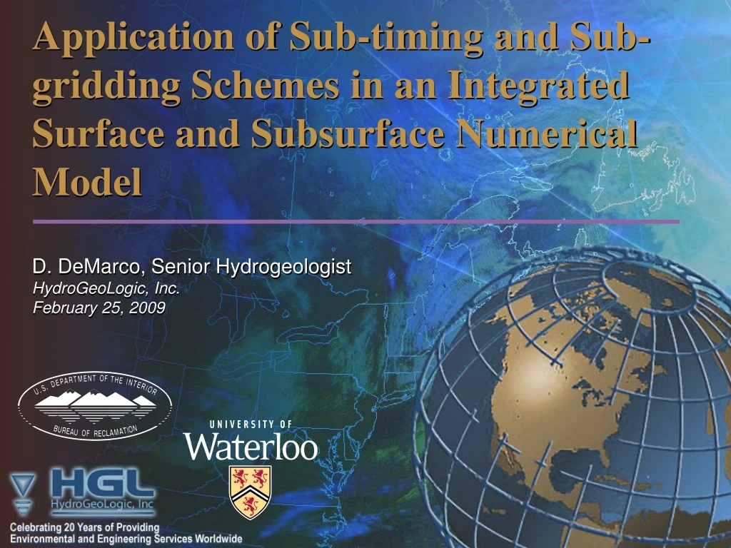
Application of Sub-timing and Sub-gridding Schemes in an Integrated Surface and Subsurface Numerical Model D. DeMarco, Senior HydrogeologistHydroGeoLogic, Inc.February 25, 2009
Contents • Integrated Surface-Subsurface Modeling • Timeline • Applications • Challenges • Resolving Challenges • Subtiming • Key Features • Results from Verification and Testing • Subgridding • Key Features • Results from Verification and Testing • Conclusions File path: O:\Projects\07_03_AOS001\Administrative\h_Meetings\June7
Timeline • Chronology of HydroGeoSphere Model Development: • Pre-1990: early subsurface models (e.g. MODFLOW) • Pre-1990: overland flow and hydrologic modeling • 1990: FRAC3DVS developed by R. Therrien/Sudicky • 1994: InHM, integrated model developed by Vanderkwaak/Sudicky • 2001: HGS: Overland flow components added to FRAC3DVS • 2003: ET, tile drains added to HGS • 2006: Subgridding & subtiming modules developed • 2008: Thermal/Temperature simulation capability added • Currently/proposed for development: • Parallelization • Subsidence • Channel Flow File path: O:\Projects\07_03_AOS001\Administrative\h_Meetings\June7
Integrated Surface-Subsurface Modeling • Accounts for all components of the hydrograph including interflow • Accurately track soil moisture storage, infiltration, and water table position • Simulate the complete hydrologic cycle • to account for all interactions between the surface and subsurface flow regimes • Simultaneously solve surface and subsurface flow & transport equations • Effective for regional and sub-regional applications File path: O:\Projects\07_03_AOS001\Administrative\h_Meetings\June7
Applications • Quantify spatial/temporal distribution of subsurface recharge, surface-subsurface interactions in streams and wetlands • Impacts of subsurface water extraction on surface water • Effects of urbanization/land-use/climate change on water quantity & quality, health of aquatic ecosystems • Restoration of adversely-impacted streams, wetlands, etc. • Subsurface versus overland migration pathways of contaminants & pathogens File path: O:\Projects\07_03_AOS001\Administrative\h_Meetings\June7
Challenges • Disparate time frames between surface/subsurface flow and transport regimes • Very large unstructured grids, irregular topography, complex boundary conditions, surface properties & geological features • Strong nonlinearities in governing equations • Data availability and upscaling issues File path: O:\Projects\07_03_AOS001\Administrative\h_Meetings\June7
Resolving Challenges • Approaches for overcoming computational burden: • Problem conceptualization • Technical expertise • Hardware innovations • Software innovations • Improved solvers/numerical approaches • Parallelization File path: O:\Projects\07_03_AOS001\Administrative\h_Meetings\June7
Resolving Challenges • "Everything that can be invented has been invented." - Charles H. Duell, Director of U.S. Patent Office, 1899 • "Theoretically, television may be feasible, but I consider it an impossibility-a development which we should waste little time dreaming about." - Lee de Forest, inventor of the cathode ray tube, 1926 • "I think there is a world market for maybe five computers." IBM's Thomas Watson, 1943 • "There is no reason anyone would want a computer in their home." Ken Olsen, Digital Equipment Corp, 1977 • “Integrated modeling is too computationally expensive.” Anonymous, 2005. File path: O:\Projects\07_03_AOS001\Administrative\h_Meetings\June7
Subtiming • Computational cost is determined by the number of discrete equations (neq) to be solved during each time step and the total # of time steps (nt). For standard FD: neq = nn • Numerical error a function of: • Δt; and • Change in h, Sw, depth of surface water • Standard FD utilizes one fixed time step for entire domain, time step size needs to satisfy the least tolerant accuracy requirement SW nodes fast temporal change requires small time step slow temporal change requires large time step Matrix nodes File path: O:\Projects\07_03_AOS001\Administrative\h_Meetings\June7
Subtiming Formulation Governing Nonlinear Flow Equation Discrete Nonlinear Equation Newton-Raphson Linearization Residual Equation with Sub-Time Stepping File path: O:\Projects\07_03_AOS001\Administrative\h_Meetings\June7
Subtiming • Subtiming applies different time step sizes to one or more subdomains • Subtiming most efficient when the hydraulic activities are high only in a small portion of the domain File path: O:\Projects\07_03_AOS001\Administrative\h_Meetings\June7
Subtiming – Example 1 • Infiltration Problem • 2m x 2m • 1cm wide macropore • 4 observation points: 3 in macropore, 1 in matrix • Simulated for 10 days • Δt = 0.25 days 1.0 days 0.25 & 1.0 days (sub-timing) • Observed pressure head at observation points File path: O:\Projects\07_03_AOS001\Administrative\h_Meetings\June7
Subtiming – Example 1 • Infiltration Problem • Solution in the sub-timed zone is as accurate as with the small time step • Small time step is ¼ the size of large time step, yet only 2.5X slower File path: O:\Projects\07_03_AOS001\Administrative\h_Meetings\June7
Subtiming –Example 2 • San Joaquin Valley model • Six drainage rivers • 7 vertical layers • 800m rectangular element • 1 day rainfall: 25 mm/day • 8 days no rainfall • Δt = 0.1 day 0.5 days 0.1 & 0.5 days (20%/100%) File path: O:\Projects\07_03_AOS001\Administrative\h_Meetings\June7
Subtiming –Example 2 • Steady-state solution obtained in 3 stages: • Steady-state surface water flow precipitation 284 mm/yr • Steady-state subsurface flow with specified head at river nodes • Integrated surface-subsurface with steady-state solution as starting condition File path: O:\Projects\07_03_AOS001\Administrative\h_Meetings\June7
Subtiming –Example 2 • San Joaquin Valley model File path: O:\Projects\07_03_AOS001\Administrative\h_Meetings\June7
Interface Elements Subgridding Concept • Localized grid refinement only in areas of interest. Does not require extending refinements vertically or laterally to model boundaries Benefit • Provide localized high resolution detail and more efficiently utilize computational resources Original Element Original Element File path: O:\Projects\07_03_AOS001\Administrative\h_Meetings\June7
Subgridding Formulation Governing Nonlinear Flow Equation Discretized Porous Medium Flow Equation Continuity of Mass Flux Across and Interface Subgridding Transformation Matrices File path: O:\Projects\07_03_AOS001\Administrative\h_Meetings\June7
Subgridding – Example 1 • Localized grid Level 1 subgridding (4 elements per original, i.e. 2 by 2) along a tributary of the Grand River. • Fine rectangular mesh shows a good representation of the 10m DEM for comparison. Fine rectangular mesh Portion of Grand River watershed File path: O:\Projects\07_03_AOS001\Administrative\h_Meetings\June7
Subgridding – Example 1 • Line contours in the left hand picture are from the fine rectangular mesh. Floods are from subgridded surface. • Note that flooded surface matches the line contours a bit better in the valley but poorly where we didn’t subgrid. Fine rectangular mesh Portion of Grand River watershed File path: O:\Projects\07_03_AOS001\Administrative\h_Meetings\June7
Subgridding – Example 1 • Level 3 subgridding (64 elements per original ,i.e. 8 by 8). Portion of Grand River watershed Fine rectangular mesh File path: O:\Projects\07_03_AOS001\Administrative\h_Meetings\June7
Subgridding – Example 1 • Flooded surface now matches line contours in river valley. Fine rectangular mesh Portion of Grand River watershed File path: O:\Projects\07_03_AOS001\Administrative\h_Meetings\June7
Subgridding – Example 1 • This shows the mesh where the tributary exits the system. Subgridding stops at depth. Fine rectangular mesh Portion of Grand River watershed File path: O:\Projects\07_03_AOS001\Administrative\h_Meetings\June7
Subgridding – Example 1 • This example is for the entire Grand river watershed with a region of fine subgridding along one river and a then a buffer of coarser subgridding. • The 2D mesh has about 3800 nodes • The 3D mesh about 100,000. File path: O:\Projects\07_03_AOS001\Administrative\h_Meetings\June7
Subgridding – Example 1 • Here is our original subregion with the fine surface for comparison. Original element Level 1 element Level 3 element Fine rectangular mesh Portion of Grand River watershed File path: O:\Projects\07_03_AOS001\Administrative\h_Meetings\June7
Subgridding – Example 2 40 Layers 1220 cm length vs. 122 cm depth 15 minutes rainfall at 25 cm/hr 1 minute no rainfall Slope: 0.01 cm 3 Cases simulated: Coarse Grid: Δx = 48.8 cm Fine Grid: Δx = 12.2 cm Subgridded: Δx = 12.2 to 48.8 cm 10/31/2019 • Infiltration Problem (Smith & Woolhiser,1971) Δx 26 File path: O:\Projects\07_03_AOS001\Administrative\h_Meetings\June7 File path: O:\Projects\07_03_AOS001\Administrative\h_Meetings\June7
Subgridding – Example 2 10/31/2019 27 File path: O:\Projects\07_03_AOS001\Administrative\h_Meetings\June7 File path: O:\Projects\07_03_AOS001\Administrative\h_Meetings\June7
Subgridding – Example 2 10/31/2019 48.8 12.2 12.2 to 48.8 28 File path: O:\Projects\07_03_AOS001\Administrative\h_Meetings\June7 File path: O:\Projects\07_03_AOS001\Administrative\h_Meetings\June7
Subgridding – Example 3 • Subgridding assigned to all model cells within 400m of major rivers, to a depth of 8 model layers. • Level 3 subgridding applied File path: O:\Projects\07_03_AOS001\Administrative\h_Meetings\June7
Subgridding – Example 3 San Joaquin River Zoom File path: O:\Projects\07_03_AOS001\Administrative\h_Meetings\June7
Subgridding – Example 3 File path: O:\Projects\07_03_AOS001\Administrative\h_Meetings\June7
Conclusions - • Integrated modeling provides a holistic and physically-based representation of the hydrologic system • Integrated surface-subsurface flow simulations typically have temporal over-discretization problems • The sub-time stepping approach can improve the efficiency of integrated simulations by applying different time step sizes to the sub-domains of different responding times File path: O:\Projects\07_03_AOS001\Administrative\h_Meetings\June7
Conclusions, cont. • Subgridding allows a relatively coarse grid to be used across the entire model domain with finer grid resolution only where needed. • Subgridding achieves optimal spatial grid resolution, improves simulation efficiency, and makes effective use of RAM File path: O:\Projects\07_03_AOS001\Administrative\h_Meetings\June7
Subtiming – Example 3 • Plot Scale Rainfall-Runoff (Abdul,1985) • Initially dry channel • 15 layers of elements • Discretization of 0.1m near surface • Critical depth boundary at entire upper surface • 50 minutes rainfall at 2 cm/hr • 50 minutes no rainfall • Δt = 25s 100s 25 & 100s File path: O:\Projects\07_03_AOS001\Administrative\h_Meetings\June7
Subtiming – Example 3 • Plot Scale Rainfall-Runoff (Abdul,1985) • Results obtained with larger time step less accurate compared to other 2 cases • Sub-timing yields an accurate solution in shortest time File path: O:\Projects\07_03_AOS001\Administrative\h_Meetings\June7
Subtiming – Example 2 • V-catchment (diGiammarco) • 1000m channel x 800m slope • Channel 10m wide • 90 minute rainfall event: 3 x 10 ˉ m/s intensity • 90 minutes: no rainfall • Manning’s roughness 0.15 and 0.015 • Δt = 150s 600s 150s & 600s 6 File path: O:\Projects\07_03_AOS001\Administrative\h_Meetings\June7
Subtiming – Example 2 • V-catchment (diGiammarco) • To achieve a similar level of accuracy for stream discharge, sub-timing is much more efficient than standard time-stepping File path: O:\Projects\07_03_AOS001\Administrative\h_Meetings\June7
Subgridding - RRR Red Rock Ranch – Subgridding Refinement File path: O:\Projects\07_03_AOS001\Administrative\h_Meetings\June7
Subtiming • Improves computational efficiency by focusing increase temporal resolution only where required • Achieves greater accuracy in areas of interest Fast Temporal Change (ie, Surface Water Flow) Requires small time step Slow Temporal Change (ie, Subsurface Water Flow) Requires large time step File path: O:\Projects\07_03_AOS001\Administrative\h_Meetings\June7