Download
1 / 27
270 likes | 362 Views
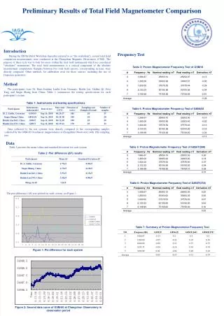
This study compares ambient concentrations with NATA model results for harmful air pollutants. Data sources include NATA NEI, ambient monitoring archives, and methodologies for calculating annual averages. The importance and relevance of NATA in assessing pollutant risks are discussed.

E N D
Preliminary Results of the 2005 NATA Model-to-Monitor Comparison Regi Oommen Emission Inventory Conference San Antonio, TX September 28, 2010
Acknowledgements • ERG Staff • Stacie Enoch • Robin Weyl • Heather Perez • Jaime Hauser • EPA • Barbara Driscoll • Ted Palma • Anne Pope
Overview • Background on NATA • Data Sources • Methodology • Preliminary Results • Conclusions
Questions to Guide the Study • Which pollutants are in good agreement between the ambient concentrations and the NATA model? • Which pollutants are under-predicted between the ambient concentrations and the NATA model? • Which pollutants are in over-predicted between the ambient concentrations and the NATA model?
Background on NATA • Conducted every three years • Began with 1996 assessment • Recently finished 4th assessment based on 2005 emissions. • Assesses cancer and/or noncancer risk for over one hundred pollutants at the census tract-level (>66,000 census tracts in U.S.). • Sector specific results (point, area nonpoint, onroad, nonroad, background, etc.) • Serves to “Bridge the Gap”
Importance of NATA – “Bridging the Gap” Benzene emission source
Importance of NATA – “Bridging the Gap” Benzene emission source Benzene monitoring site
Data Sources - NATA • 2005 NATA • For this analysis, specific receptor locations were modeled for over 100 HAPs. • Improved understanding of secondary formation and transformation of important HAPs (formaldehyde, acetaldehyde, acrolein, 1,3-butadiene). • Coke oven facilities: Emissions buoyancy accounted for. • Dose-response factors/unit risk estimates updated.
Data Sources – NATA NEI • 2005 NATA National Emissions Inventory (NEI) • All sectors (point, area nonpoint, onroad, nonroad, biogenic) • Criteria and HAPs • Primarily state/local/tribal data. Also integrates emissions data from EPA/other federal programs: • Clean Air Markets Division (CAMD) • Risk and Technology Review (RTR) • Toxic Release Inventory • Other studies (trade associations, Bureau of Ocean Energy Management, Regulatory, and Enforcement)
Data Sources – NATA NEI • 2005 NATA National Emissions Inventory • Several improvements compared to previous inventories • RTR and Lead NAAQS revisions were incorporated. • Certain nonpoint source categories disaggregated to point sources inventory (chrome plating, forest and wildfires). • Data from airports (19,000+) were added • MOVES model used for certain mobile source HAPs • Landfill emissions adjusted/removed
Data Sources – Ambient Monitoring • Phase VI Ambient Monitoring Archive • Ambient monitoring archive of over 26 million HAP records • Timeframe: 1973-2007 • 2005 year: 2.9 million HAP records. Composed of data from: • EPA’s Air Quality Subsystem (92%) • Interagency Monitoring of Protected Visual Environments (IMPROVE) (7%) • Phase V historical archive (1%)
Methodology • Calculating Annual Averages • Emission estimates are for an entire year • NATA model develops annual average concentrations • Procedure • Step 1: Extract 2005 ambient HAP data from the Phase VI archive. • Step 2: For sub-daily measurements (hourly, etc.), calculate valid daily measurements. • Step 3: Identify daily concentrations (by HAP, by site) which represent an entire year. • Step 4: Calculate annual average by HAP by site from the valid daily averages.
Methodology • Averaging Criteria – Valid Daily Averages • Sub-daily measurements must have minimum 75% temporal coverage within a day: • Minimum eighteen 1-hour detected measurements • Minimum six 3-hour detected measurements • Minimum five 4-hour detected measurements • Use zero as a surrogate for non-detects
Methodology • Averaging Criteria – Valid Quarterly coverage • Calendar quarter must have minimum 75% temporal coverage within a quarter: • Quarters are: January-March, April-May, June-August, September-December. • Minimum six pre-described sub-quarter zones with a valid daily average. • Sites sampling 1-in-12 days will have 7 or 8 samples within a quarter. More intensive sampling (1-in-6 days or 1-in-3 days) will have more opportunity to meet this criteria.
Methodology • Averaging Criteria – Annual Average • Annual average must have minimum 75% temporal coverage within a year (i.e., three valid quarters) • If all criteria are met, average the valid daily concentrations and non-detects using zero as a surrogate.
Methodology • Model-to-Monitor Comparison • Simply divide model concentration by annual average concentration for each HAP and monitor. • Statistical distributions (minimum 25 monitors by HAP): • 25th, 50th, and 75th percentiles • Average • Percent monitors within 10%, 20%, and 30% • Percent monitors within Factor of 2 • Percent monitors under-estimated • Percent monitors over-estimated
Preliminary Results – Gaseous HAPs (>100 monitors) Within Factor of 2 75th percentile Mean Median 25th percentile
Preliminary Results – Gaseous HAPs (25-100 monitors) Within Factor of 2 75th percentile Mean Median 25th percentile
Preliminary Results – PM10 HAPs 75th percentile Within Factor of 2 Mean Median 25th percentile
Preliminary Results • Overall: • 5,400+ model-to-monitor comparisons • 9% of all median ratios were between 0.9 and 1.1 • 17%....were between 0.8 and 1.2 • 25%....were between 0.7 and 1.3 • 44%....were within a Factor of 2 • Carbon tetrachloride, methyl chloride and arsenic (PM10) had median ratios between 0.9 to 1.1 • Interquartile range within Factor of 2 for acetaldehyde, arsenic (PM10), benzene, carbon tetrachloride, formaldehyde, methyl chloride, and toluene.
Preliminary Results • Under-prediction (75th percentile < Factor of 2) for 13 HAPs: • Ethylene dichloride • n-Hexane • 1,1,2-Trichloroethane • Acrylonitrile • Carbon disulfide • Chloroprene • 1,3-Dichloropropene • Over-prediction (25th percentile > Factor of 2) for 1 HAP: • Beryllium (PM10) • Ethylidene dibromide • Ethylene dichloride • Methyl isobutyl ketone • Propionaldehyde • Propylene dichloride • Vinylidene chloride
Data Considerations • These are preliminary results. • Uncertainties: • Emissions characterization (i.e, location, emission rates, release parameters) • Meteorological characterizations (i.e., representativeness) • Model formulation and methodology (i.e., dispersion, plume rise, deposition) • Monitoring uncertainties (i.e., questions about acrolein, annual averaging techniques, etc.) • Background concentrations (i.e., representativeness)
Data Considerations • Under-estimation: • NATA NEI may be missing specific emission sources • Emission rates may be under-estimated • Monitoring data/sampling methods/non-detects/averaging techniques • Background concentrations poorly characterized
Conclusion • Which pollutants are in good agreement between the ambient concentrations and the NATA model? • Acetaldehyde • Arsenic (PM10) • Benzene • Carbon tetrachloride • Formaldehyde • Methyl chloride • Toluene
Conclusion • Which pollutants are under-predicted between the ambient concentrations and the NATA model? • Ethylene dichloride • n-Hexane • 1,1,2-Trichloroethane • Acrylonitrile • Carbon disulfide • Chloroprene • 1,3-Dichloropropene • Which pollutants are over-predicted between the ambient concentrations and the NATA model? • Beryllium (PM10) • Ethylidene dibromide • Ethylene dichloride • Methyl isobutyl ketone • Propionaldehyde • Propylene dichloride • Vinylidene chloride