Two Independent Populations (Chapter 6)
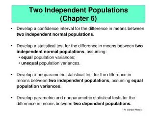
Two Independent Populations (Chapter 6). Develop a confidence interval for the difference in means between two independent normal populations . Develop a statistical test for the difference in means between two independent normal populations , assuming: equal population variances;

Two Independent Populations (Chapter 6)
E N D
Presentation Transcript
Two Independent Populations (Chapter 6) • Develop a confidence interval for the difference in means between two independent normal populations. • Develop a statistical test for the difference in means between two independent normal populations, assuming: • equal population variances; • unequal population variances. • Develop a nonparametric statistical test for the difference in means between two independent populations, assuming equal population variances. • Develop parametric and nonparametric statistical tests for the difference in means between two dependent populations.
Situation Need to determine if concentration of contaminant at an old industrial site is greater than background levels from areas surrounding the site. Take soil samples at random locations within the site and at random locations at areas outside the site. Assume values at areas outside the site are unaffected by site activities that lead to contamination.
Hypotheses of Interest 1. Background level of contaminant is greater than the no-detect level (-5.0) [on a natural log scale]. 2. Site level of contaminant is greater than the no-detect level (-5.0). 3. Site level is different from Background level. Is the situation this or this? 2 1 2 -5.0
One- Sample Hypothesis Tests Background level of contaminant is greater than the no-detect level (-5.0). Site level of contaminant is greater than the no-detect level (-5.0). H0: mi£ -5.0 HA:mi> -5.0 i = 1 => Background areas (B) i = 2 => Contamination site (S) One sided t-tests: Critical Values T. S. n t.05,n-1 7 1.943 8 1.895 9 1.860 10 1.833 R.R.
DATA and One-Sided T-tests Y -2.96 -1.09 -3.13 -2.12 -2.59 -4.31 -1.20 H0: mB£ m0 = -5.0 HA: mB > m0 = -5.0 Pr(Type I error) = a = 0.05 T.S. Reject H0 if t > ta,n-1 T0.05,6=1.943 R.R. Conclusion: Since 5.90 > 1.943 we reject H0 and conclude that the true average background level is above -5.0. Same test could be performed for contaminated site data.
Comparison Hypothesis H0: Site level is not different from Background level. (mB = mS) HA: Site level is different from Background level. (mB ¹ mS) This requires comparing sample means from two “independent” samples, one from each population. T. S. Obvious test statistic. the standard error of the difference of the two means.
Standard Error of the Difference of Two Means If the true variances of the two populations are known, we use the property of independent random variables that says: Var(X-Y) = Var(X) + Var(Y) . From sampling Dist of From sampling Dist of T. S.
Assume the two populations have the same, or nearly the same true variance, s2p. True standard error of the difference of two means. Estimate of the standard error of the mean differences. Estimate of the common (Pooled) standard deviation.
Confidence Interval for difference Assume confidence level of (1-)100%
Statistical test for difference of means Pooled Variances T-test Pr(Type I Error) = Test Statistic:
CONT YBYS -2.96 -3.81 -1.09 -5.83 -3.13 -5.70 -2.12 -4.11 -2.59 -3.83 -4.31 -5.01 -1.20 -5.49 Background Site H0: mB - mS = 0 HA: mB - ms 0 HA: Average site level significantly different from background.
Pr(Type I Error) = a = 0.05 T.S. Reject if: R.R. Conclusion: Since 4.304 > 2.179 we reject H0 and conclude that site concentration levels are significantly different from background.
Separate Variances CI and T-test What if the two populations do not have the same variance? • New estimate of standard error of difference. • Test and CI is no longer exact - uses Satterthwaite’s approximate df value (df’). C.I.: T.S.: Round df’ down to the nearest integer.
Redo Test For site contamination example, assume s1s2 and redo test. T.S. R.R. Reject if: Since 4.304 > 2.201 we reject H0 and conclude that site concentration levels are significantly different from background. Conclusion:
Sample Size Determination (equal variances) (1-)100% CI for μ1 – μ2: = Pr(Type I Error) = Pr(Type II Error) One-sided Test: Two-sided Test:
Example of Sample Size Determination In our sample, a D of 2.34 was observed. What if we had wanted to be sure that a D of say 1 unit would be declared significant with: 0.05 = = Pr(Type I Error) 0.10 = = Pr(Type II Error) Assume a common population variance of s2 = 1. One-sided test: Two-sided test: n=n1=n2
Summary • These two-sample inferences require the assumption of independent, normal population distributions. • If we have reason to believe the two population variances are equal, then we should use the pooled variances method. This results in more powerful inferences. • We need not worry about the normality assumption when both sample sizes are large, all results are still approximately correct. (CLT.) • What to do when independence does not hold? Advanced! Partial solution next lecture (paired samples). • What to do when we have small samples and we don’t believe the data are normal? Next slide…
The Wilcoxon Rank Sum Test A class of nonparametric tests. These: • Do not require data to have normal distributions. • Seek to make inferences about the median, a more appropriate representation of the center of the population for highly skewed and/or very heavy-tailed distributions. In the Wilcoxon Rank SumTest: • Population variances assumed to be equal. • Measurements (observations) are assumed to be independent from continuous distributions. • Interest is whether the center of the two population distributions are the same or not. • Also known as the Mann-Whitney U Test. • 1-sample equivalent: Wilcoxon Signed RankTest.
Idea behind the Wilcoxon Test H0: Populations are identical If H0 is true, when we put the data from the two samples together and sort them from lowest to highest, i.e. we rank them (lowest obs gets rank=1, 2nd rank=2, etc., tied obs get average of ranks). The ranks of the observations from the two samples should be fairly well intermingled. Thus, the sum of the ranks from population 1 observations should be approximately equal to the sum of the ranks of population 2 observations. HA: Population 1 is shifted to the right of population 2. If HA is true, if we put the data from the two samples together then sort them lowest to highest, the sum of the ranks of population 1 observations should be greater than the sum of ranks of observations from population 2 .
Definition of Population 1 NOTE: Population 1 should be taken to be the one corresponding to the smaller sample size (n1 n2). If the sample sizes are equal (n1=n2), either one can be Population 1. This is so that the Tables in Ott will give correct critical values. (Ott inadvertantly does not mention this!)
Wilcoxon Test Statistic Let T denote the sum of the ranks of population 1 observations. T.S. If n110 and n2 10 use T as the test statistic and Table 5 in Ott & Longnecker for critical values. Situation #1 1. Reject H0 if T > TU 2. Reject H0 if T < TL 3. Reject H0 if T>TU or T<TL R.R. H0: Populations are identical HA: 1. Population 1 is shifted to right of population 2. 2. Population 1 is shifted to the left of population 2. 3. Populations 1 and 2 have different location parameters.
Situation #2 1. Reject H0 if z > z 2. Reject H0 if z < -z 3. Reject H0 if |z|>z /2 = Pr(Type I Error) R.R. If n1>10, n2 >10 we use a normal approximation to the distribution of the sum of the ranks. Let T denote the sum of the ranks of population 1 observations. T.S. and tj denotes the number of tied ranks in the jth group of ties, j=1,…,k.
Situation #1: Group Value Rank Pop 1 Ranks 1 -1.09 14 14 1 -1.20 13 13 1 -2.12 12 12 1 -2.59 11 11 1 -2.96 10 10 1 -3.13 9 9 2 -3.81 8 2 -3.83 7 2 -4.10 6 1 -4.31 5 5 2 -5.01 4 2 -5.41 2.5 2 -5.41 2.5 2 -5.83 1 SUM 74 = T n110 and n2 10 Two sided alternative hypothesis R.R. :Reject H0 if T>TU or T<TL Table 5 n1 = n2 = 7 TL = 37 TU = 68 Conclusion: Reject H0
Wilcoxon Critical Values Table 5
Confidence Interval for Δ= μ1 – μ2 Can be constructed in analogous way to the nonparametric CI for μbased on the Sign Test. (See §6.3 in Ott.)
Paired Data Situation (§6.4-6.5) In this set of slides we will: • Develop confidence intervals and test for the difference between two means that have been measured on the same or highly related experimental units. • The underlying population of differences is assumed to be normally distributed. • A nonparametric alternative that does not rely on normality will be discussed (§6.5).
Situation Two analysts, supposedly of identical abilities, each measure the parts per million of a certain type of chemical impurity in drinking water. It is claimed that analyst 1 tends to give higher readings than analyst 2. To test this theory, each of six water samples is divided and then analyzed by both analysts separately. The data are as follows: Data are paired hence observations are not independent. Observations in the same row are more likely to be close to each other than are observations between rows.
Paired Data Considerations Because of the dependence within rows we don’t use the difference of two means but instead use the mean of the individual differences. written as Let yij represent the ith observation for the jth sample, i=1,…,n, j=1,2. Compute di = yi1 - yi2 the difference in responses for the ith observation, and then proceed as in the one sample t-test situation. the sample mean of the differences. the sample standard deviation of the differences.
Importance of Independence/Dependence on Variance of Difference If the two populations were independent, the variance of the difference would be computed using the probability rule: Var( X - Y ) = Var(X) + Var(Y) But here the two populations are dependent and the above rule does not hold. i.e we don’t use a pooled variance estimator. We use the variance of the differences. Hence In above Example: Very different!
The paired t-test H0: d = D0 Ha: 1. d > D0 2. d < D0 3. d D0 Test Statistic: Rejection Region: 1. Reject H0 if t > t,n-1 2. Reject H0 if t < -t ,n-1 3. Reject H0 if |t| > t /2,n-1 -level confidence interval: For the Example, t = 1.853 and t0.05,5 = 2.015 hence we do not reject H0: d =0 in testing situation 1, and conclude that there are no significant differences. 95% CI: 1.4 1.94 or ( -.54 , 3.34 )
Wilcoxon Signed-Rank Test for Paired Data (§6.5) • A nonparametric alternative to the paired t-test when the population distribution of differences are not normal. (Requires symmetry about the population median of the differences, M.) • Test Construction: • Compute the differences in the pairs of observations. • Let D0 be the hypothesized value of M, and subtract D0 from all the differences. • Delete all zero values, and let n be the resulting number of nonzero values. • List the absolute values in increasing order, and assign them ranks 1,…,n (or average of ranks for ties). T+ = sum of the positive ranks (T+ = 0 if no positive ranks). T- = sum of the negative ranks (T- = 0 if no negative ranks).
R.R. 1. Reject if TT,n 2. Reject if T T,n 3. Reject if T T/2,n Situation 1: Small Sample (n≤50) H0: M = D0 (usually 0). HA: 1. M > D0. 2. M < D0. 3. M ≠ D0. T.S. 1. T=T- 2. T=T+ 3. T=smaller(T-,T+) Critical values (from Table 6)
T.S. R.R. 1. Reject H0 if z > z 2. Reject H0 if z < - z 3. Reject H0 if |z| > z /2 H0: M = D0 (usually 0). HA: 1. M > D0. 2. M < D0. 3. M ≠ D0. Situation 2: Large Sample (n>50) g = number of distinct ranks assigned to the differences. (If no ties, g=n.) tj = number of tied ranks in jth group. (If no ties, tj=1 for j=1,…,g, and the summation term is zero.) Critical values (from Table 1)
Back to the Problem Differences Ranks (signs) -1.3 1 (-) -0.1 2 (-) 1.5 3.5 (+) 1.5 3.5 (+) 3.3 5 (+) 3.4 6 (+) • For HA: M > 0 (1st case): • the test statistic is T- = 3; • the critical value is T0.05,6 = 2. • Hence we do not reject H0 and conclude that analyst 1 does not tend to give higher readings than analyst 2.
Illustration of calculationssupposing the problem were of a large sample nature (not the case here). Differences Ranks (signs) -1.3 1 (-) -0.1 2 (-) 1.5 3.5 (+) 1.5 3.5 (+) 3.3 5 (+) 3.4 6 (+) For HA: M > 0, test statistic is Z = (T+ – μT) / σT = (18 – 10.5) / 4.8 =1.6 Since z = 1.6 < z0.05 = 1.645, we do not reject H0.
Concluding Comments The paired measurements (samples) case can be extended to more than two measurements; called repeated measurements. When repeated measurements are taken on an individual, we are in the same situation as with two paired samples, that is, the repeated measurements on an individual are expected to be more correlated than measurements among individuals. Solutions to the repeated measurements case cannot follow the simple solution for two dependent samples. The final solution involves specifying not only what we expect to happen in the means of the sampling “times” but we have to specify the structure of the correlations between sampling times. It is advantageous to design a paired data experiment rather than an independent samples one. This helps to eliminate the confounding effect (masking of treatment differences) that sources of variation other than the treatments have on the experimental units.