Download
1 / 38
390 likes | 597 Views
General Purpose Procedures Applied to Scheduling. Contents Constructive approach 1. Dispatching Rules Local search 1. Simulated Annealing 2. Tabu-Search 3. Genetic Algorithms. Constructive procedures : 1. Dispatching Rules 2. Composite Dispatching Rules 3. Dynamic Programming

E N D
General Purpose ProceduresApplied to Scheduling Contents Constructive approach 1. Dispatching Rules Local search 1. Simulated Annealing 2. Tabu-Search 3. Genetic Algorithms
Constructive procedures: 1. Dispatching Rules 2. Composite Dispatching Rules 3. Dynamic Programming 4. Integer Programming 5. Branch and Bound 6. Beam Search Local Search 1. Simulated Annealing 2. Tabu-Search 3. Genetic Algorithms Heuristic technique is a method which seeks good (i.e. near-optimalsolutions) at a reasonable cost without being able to guaranteeoptimality.
Dispatching Rules • A dispatching rule prioritises all the jobs that are waiting forprocessing on a machine. • Classification • Static: not time-dependent • Dynamic: time dependent • Local: uses information about the queue where the job is waiting or machine where the job is queued • Global: uses information about other machines (e.g. processing time of the jobs on the next machine on its route, or the current queue length
Local Search Step. 1. Initialisation k=0 Select a starting solution S0S Record the current best-known solution by setting Sbest = S0 and best_cost = F(Sbest) Step 2. Choice and Update Choose a Solution Sk+1N(Sk) If the choice criteria cannot be satisfied by any member of N(Sk), then the algorithm stops if F(Sk+1) < best_cost then Sbest = Sk+1 and best_cost = F(Sk+1) Step 3. Termination If termination conditions apply then the algorithm stops else k = k+1 and go to Step 2.
Global Optimum: better than all other solutions • Local Optimum: better than all solutions in a certain neighbourhood
1. Schedule representation • 2. Neighbourhood design • 3. Search process • 4. Acceptance-rejection criterion • 1. Schedule representation • Nonpreemptive single machine schedule • permutation of n jobs • Nonpreemptive job shop schedule • m consecutive strings, each representing a permutation ofn operations on a machine
2. Neighbourhood design • Single machine: • adjacent pairwise interchange • take an arbitrary job in the schedule and insert it in another positions • Job shop: • interchange a pair of adjacent operations on the critical path of the schedule • one-step look-back interchange
current schedule (h, l) (h, k) machine h (i, j) (i, k) machine i • schedule after interchange of (i, j) and (i, k) (h, l) (h, k) machine h (i, k) (i, j) machine i • schedule after interchange of (h, l) and (h, k) (h, k) (h, l) machine h (i, k) (i, j) machine i
3. Search process • select schedules randomly • select first schedules that appear promisingfor example, swap jobs that affect the objective the most • 4. Acceptance-rejection criterion • probabilistic: simulated annealing • deterministic: tabu-search
Simulated Annealing Contents 1. Basic Concepts 2. Algorithm 3. Practical considerations
t Basic Concepts • Allows moves to inferior solutions in order not to get stuck in a poor local optimum. • c = F(Snew) - F(Sold) F has to be minimized inferior solution (c > 0) still accepted if U is a random number from (0, 1) interval t is a cooling parameter: t is initially high - many moves are accepted t is decreasing - inferior moves are nearly always rejected • As the temperature decreases, the probability of accepting worse moves decreases. c > 0 inferior solution -c < 0
Algorithm Step 1. k=1 Select an initial schedule S1 using some heuristic and set Sbest = S1 Select an initial temperature t0 > 0Select a temperature reduction function (t) Step 2. Select ScN(Sk) If F(Sbest) < F(Sc) If F(Sc) < F(Sk) then Sk+1 = Sc else generate a random uniform number Uk If Uk < then Sk+1 = Sc else Sk+1 = Sk else Sbest = Sc Sk+1 = Sc
Step 3. tk = (t) k = k+1 ; If stopping condition = true then STOP else go to Step 2
Exercise. Consider the following scheduling problem 1 | dj | wjTj . Apply the simulated annealing to the problem starting out with the3, 1, 4, 2 as an initial sequence. Neighbourhood: all schedules that can be obtained throughadjacent pairwise interchanges. Select neighbours within the neigbourhood at random. Choose (t) = 0.9 * t t0 = 0.9 Use the following numbers as random numbers: 0.17, 0.91, ...
Sbest= S1 = 3, 1, 4, 2 F(S1) = wjTj = 1·7 + 14·11 + 12·0+ 12 ·25 = 461 = F(Sbest) t0 = 0.9 Sc = 1, 3, 4, 2 F(Sc) = 316 < F(Sbest) Sbest= 1, 3, 4, 2 F(Sbest) = 316 S2 = 1, 3, 4, 2 t = 0.9 · 0.9 = 0.81 Sc = 1, 3, 2, 4 F(Sc) = 340 > F(Sbest) U1 = 0.17 > = 1.35*10-13 S3= 1, 3, 4, 2 t = 0.729
Sc = 1, 4, 3, 2 F(Sc) = 319 > F(Sbest) U3 = 0.91 > = 0.016 S4= S4 = 1, 3, 4, 2 t = 0.6561 ...
Practical considerations • Initial temperature • must be "high" • acceptance rate: 40%-60% seems to give good results in many situations • Cooling schedule • a number of moves at each temperature • one move at each temperature • t = ·t is typically in the interval [0.9, 0.99] is typically close to 0 • Stopping condition • given number of iterations • no improvement has been obtained for a given number of iteration
Tabu Search Contents 1. Basic Concepts 2. Algorithm 3. Practical considerations
Basic Concepts Tabu-lists contains moves which have been made in the recent past butare forbidden for a certain number of iterations. Algorithm Step 1. k=1 Select an initial schedule S1 using some heuristic and set Sbest = S1 Step 2. Select ScN(Sk) If the move Sk Sc is prohibited by a move on the tabu-list then go to Step 2
If the move Sk Sc is not prohibited by a move on the tabu-list then Sk+1 = Sc Enter reverse move at the top of the tabu-list Push all other entries in the tabu-list one position down Delete the entry at the bottom of the tabu-list If F(Sc) < F(Sbest) then Sbest = Sc Go to Step 3. Step 3. k = k+1 ; If stopping condition = true then STOP else go to Step 2
Example. 1 | dj | wjTj Neighbourhood: all schedules that can be obtained throughadjacent pairwise interchanges. Tabu-list: pairs of jobs (j, k) that were swapped within the lasttwo moves S1 = 2, 1, 4, 3 F(S1) = wjTj = 12·8 + 14·16 + 12·12 + 1 ·36 = 500 = F(Sbest) F(1, 2, 4, 3) = 480 F(2, 4, 1, 3) = 436 = F(Sbest) F(2, 1, 3, 4) = 652 Tabu-list: { (1, 4) }
S2 = 2, 4, 1, 3, F(S2) = 436 F(4, 2, 1, 3) =460 F(2, 1, 4, 3) (= 500) tabu! F(2, 4, 3, 1) = 608 Tabu-list: { (2, 4), (1, 4) } S3 = 4, 2, 1, 3, F(S3) = 460 F(2, 4, 1, 3) (=436)tabu! F(4, 1, 2, 3) = 440 F(4, 2, 3, 1) = 632 Tabu-list: { (2, 1), (2, 4) } S4 = 4, 1, 2, 3, F(S4) = 440 F(1, 4, 2, 3) =408 = F(Sbest) F(4, 2, 1, 3) (= 460) tabu! F(4, 1, 3, 2) = 586 Tabu-list: { (4, 1), (2, 4) } F(Sbest)= 408
Practical considerations • Tabu tenure: the length of time t for which a move is forbiden • t too small - risk of cycling • t too large - may restrict the search too much • t=7 has often been found sufficient to prevent cycling • Number of tabu moves: 5 - 9 • If a tabu move is smaller than the aspiration level then we accept the move
Genetic Algorithms Contents 1. Basic Concepts 2. Algorithm 3. Practical considerations
Basic Concepts Simulated AnnealingTabu Search Genetic Algorithms versus • a single solution is carried over from one iteration to the next • population based method • Individuals (or members of population or chromosomes) individuals surviving from the previous generation + children generation
Fitnessof an individual (a schedule) is measured by the value of the associated objective function • Representation • Example. • the order of jobs to be processed can be represented as a permutation:[1, 2, ... ,n] • Initialisation • How to choose initial individuals? • High-quality solutions obtained from another heuristic technique can help a genetic algorithm to find better solutions more quickly than it can from a random start.
Reproduction • Crossover: combine the sequence of operations on one machine in one parent schedule with a sequence of operations on another machine in another parent. • Example 1. Ordinary crossover operator is not useful! Cut Point P1 = [2 1 3 4 5 6 7] P2 = [4 3 1 2 5 7 6] O1 = [2 1 3 2 5 7 6] O2 = [4 3 14 5 6 7] Example 2. Partially Mapped Crossover Cut Point 1 Cut Point 2 31 42 55 P1 = [2 134 5 6 7] P2 = [43125 7 6] O1 = [43 12 5 6 7] O2 = [21 345 7 6]
Example 3. Preserves the absolute positions of the jobs taken from P1and the relative positions of those from P2 Cut Point 1 P1 = [2 1 3 4 5 6 7] P2 = [4 3 1 2 5 7 6] O1 = [2 14 3 5 7 6] O2 = [4 3 2 1 5 6 7] Example 4. Similar to Example 3 but with 2 crossover points. Cut Point 1 Cut Point 2 P1 = [2 1 3 4 5 6 7] P2 = [4 3 12 5 7 6] O1 = [3 4 5 1 2 7 6]
Mutation enables genetic algorithm to explore the search space not reachable by the crossover operator. • Adjacent pairwise interchange in the sequence [1,2, ... ,n] [2,1, ... ,n] Exchange mutation: the interchange of two randomly chosen elementsof the permutation Shift mutation: the movement of a randomly chosen element a random number of places to the left or right Scramble sublist mutation: choose two points on the string in randomand randomly permuting the elements between these two positions.
slice for the 1st individual selected individual slice for the 2nd individual . . . • Selection • Roulette wheel: the size of each slice corresponds to the fitness of the appropriate individual. Steps for the roulette wheel 1. Sum the fitnesses of all the population members, TF 2. Generate a random number m, between 0 and TF 3. Return the first population member whose fitness added to the preceding population members is greater than or equal to m
Tournament selection • 1. Randomly choose a group of T individuals from the population. • 2. Select the best one. • How to guarantee that the best member of a population will survive? • Elitist model: the best member of the current population is set to be a member of the next.
Algorithm Step 1. k=1 Select N initial schedules S1,1 ,... ,S1,N using some heuristic Evaluate each individual of the population Step 2. Create new individuals by mating individuals in the current populationusing crossover and mutation Delete members of the existing population to make place forthe new members Evaluate the new members and insert them into the population Sk+1,1 ,... ,Sk+1,N Step 3. k = k+1 If stopping condition = true then return the best individual as the solution and STOP else go to Step 2
Example • 1 || Tj • Population size: 3 • Selection: in each generation the single most fit individual reproduces using adjacent pairwise interchange chosen at random there are 4 possible children, each is chosen with probability 1/4 Duplication of children is permitted. Children can duplicate other members of the population. • Initial population: random permutation sequences
Generation 1 • Individual 25314 14352 12345 • Cost 25 17 16 • Selected individual: 12345 with offspring 13245, cost 20 • Generation 2 • Individual 13245 14352 12345 • Cost 20 17 16 • Average fitness is improved, diversity is preserved • Selected individual: 12345 with offspring 12354, cost 17 • Generation 3 • Individual 12354 14352 12345 • Cost 17 17 16 • Selected individual: 12345 with offspring 12435, cost 11
Generation 4 • Individual 14352 12345 12435 • Cost 17 16 11 • Selected individual: 12435 • This is an optimal solution. • Disadvantages of this algorithm: • Since only the most fit member is allowed to reproduce (or be mutated) the same member will continue to reproduce unless replaced by a superior child.
Practical considerations • Population size: small population run the risk of seriously under-covering the solution space, while large populations will require computational resources. Empirical results suggest that population sizes around 30 are adequate in many cases, but 50-100 are more common. • Mutation is usually employed with a very low probability.
Summary • Meta-heuristic methods are designed to escape local optima. • They work on complete solutions. However, they introduce parameters (such as temperature, rate of reduction of the temperature, memory, ...) How to choose the parameters? • Other metaheuristics • Ant optimization • GRASP