Download
1 / 28
290 likes | 376 Views
Explore the critical behavior and dynamics of Ising spin glasses through numerical definitions, equations, and analysis of dynamical exponents. Understand the temperature-dependent properties and fluctuations in these systems. Collaboration with Helmut Katzgraber and Michel Pleimling.

E N D
Critical behaviour and dynamics of Ising spin glasses Ian Campbell LCVN Universite Montpellier II Collaborations with - Helmut Katzgraber, ETH Zurich and - Michel Pleimling, Erlangen
Numerical Definition of the dynamical exponent z(T) (Katzgraber and Campbell PRB 72 (2005) 014462) At Tc ceq(L) ~ L{2-h} in equilibrium and cne(t) ~ t{(2-h)/zc} as function of anneal time t following a quench to Tc . So at Tc we can define an anneal time dependent length scale L*(t) = At{1/zc} Quite generally, if at any temperature T the equilibrium SG susceptibility as a function of sample size L is ceq(L,T), and the non-equilibrium SG susceptibility after at anneal time t after a quench to temperature T is cne(t,T) for a large sample of size Lb, then an infinite sample size time dependent length scale L*(t) can be rigourously defined by writing the implicit equation : cne(L*(t),T)=ceq(L,T) [as long as L*(t) << Lb.] L*(t,T) is about twice the correlation length l(t) as one could expect.
From the measured values of L*(t,T) we find numerically that an equation having the same functional form as at criticality L*(t,T) = A(T)t{1/z(T)} with a temperature dependent effective exponent z(T) and a weakly temperature dependent prefactor A(T) gives an excellent parametrization of ISG and GG data in each system, not only at temperatures below T_c (confirming the conclusions of Kisker et al 1996 and Parisi et al 1996}) but also above T_c. z(T) varies smoothly through SG transition temperatures. Energy data can be analysed just the same way as c data and give consistent results for z(T).
red : c(L) black : c(t) transposed to c(L*(t)) using L*(t)=A(T)t{1/z(T)} 2d GG T=0.173
Energy-susceptibility relation Red : [e(L)-e(inf)] against c(L) Black : [e(t)-e(inf)] against c(t) (not a fit !) 2d GG T = 0.173
Conclusion #1 For Ising and vector SGs, the dynamic exponent z(T) can be defined for the entire range of temperatures, not only at Tc but also well below and well above. zc is just one particular value, z(T=Tc). z(T) varies smoothly through spin glass transitions PRB 72 (2005) 014462
Estimation of Tc in ISGs Standard method is to use the Binder cumulant crossing point. Accurate in 4d, but in 3d this is subject to large corrections to scaling. Similardifficulties for x(L)/L. Alternatively combine static and dynamic measurements (1995): - c(L) ~ L{2-h} in equilibrium at Tc - c(t) ~ t{(2-h)/z)} after quench to Tc - C(t) ~ t{-(d-2+h)/2z} after a long anneal at Tc The three measurements are consistent at only one temperature, which must be Tc, and from the values at Tc one gets h and zc. Recent high temperature series results for Tc in 4d ISGs are in excellent agreement with numerical values using this method.
Conclusion #2 The consistency method gives accurate and reliable estimates for Tc confirmed by high T series calculations. The values of the associated exponents h and zc from the same simulations can also be taken to be accurate. PRB 72 (2005) 092405
Dynamic exponents [see Henke and Pleimling 2004] Definitions : Anneal for a time s, measure at time t (>s) At criticality T=Tc, measure - Autocorrelation function decay after quench (no anneal) : C(t,s=0) ~ t^{-lc/zc} where -lc/zc = d/zc - qcqc being an independent dynamic exponent , the “initial slip”. - Fluctuation-dissipation ratio : response R(t,s)= [ d<Si(t)>/dh(s) ] {h=0} (t>>s) gives FD ratio X(t,s) =TR(t,s)/(dC(t,s)/ds)
Autocorrelation relaxation after quench to Tc 3d ISG fluctuation-dissipation ratio at Tc Interaction distributions b : Binomial g : Gaussian l : Laplacian Pleimling et al cond-mat/0506795 (cf Malte Henkel)
3d ISGs : derivative of the autocorrelation function decay without anneal (s=0) at Tc
Conclusion #3 The dynamic exponents zc, X(infinity), lc/zc (and the static exponent h) are not universal in ISGs. cond-mat/0506795
What about n ? The consistency method gives reliable values of Tc, h, and z. To determine the exponent n needs data not at Tc but at T > Tc The critical divergences x ~ {T-Tc} -n, c ~ {T-Tc} -g etc are generally quoted in textbooks (and many papers) as x ~ {t} -nc ~ {t} -g with the scaling variable t = (T-Tc)/Tc Is this the right scaling variable ? For c in canonical ferromagnets the range of temperature over which the critical temperature dependence remains a good approximation can be considerably extended by writing c ~ {t} -gwith t = (T-Tc)/T as the scaling variable (as proposed by Jean Soultie).
Note that t = 1 means T = infinity, while t = 1 means only T = 2Tc i.e. with t as the scaling variable, the range of critical behaviour c(t) ~ {t} -g extends as a good approximation to infinite T, while with t as scaling variable the critical region is very limited. Why ? Look at high series work. In ferromagnets, the exact high temperature series for c(b) is an expansion in powers of b (=1/T) c(b) = 1 + {a1}b + {a2}b2 +..... with the an determined exactly up to n = 25 by combinatorial methods in 3d ( Butera and Comi) and up to n=325 in 2d (Nickel). ***********
A fundamental mathematical identity is Darboux’s first theorem (1878) : (1-x) -g = 1 + gx + {g(1+g)/2}x2 + {g(1+g)(2+g)/6}x3 +... i.e. = 1 + a1x + a2x2 + a3x3 + ... with a{n}/a{n-1} = [n+g-1]/[n] Now {t} -g = [(T-Tc)/T] -g = {1-b/bc} -g (b = 1/T) If c(b) is to behave as {1-b/bc} -g over the whole range of T, then the combinatorial series of an must be 1, a1, a2, ... such that rn= an/a(n-1) = (1+(g-1)/n)/bc It turns out that this works remarkably well down to quite small n ( hence to high T) for the standard Ising ferromagnets (2d, 3d sc, bcc, fcc....)
So what about spin glasses ? The high T ISG combinatorial series take the form (Daboul et al) c(b) = 1 + a1b2 +a2b4 + a3b6 + ....... ( powers of b2 instead of b) So following the same argument as for the ferromagnet but replacing b by b2 , the appropriate scaling form for the ISG c should be c(b) = (1-b2/bc2) -g [(1-b2/bc2) => 2(1-b/bc) at T ~ Tc so so critical scaling is OK] With the data available for the moment, this also works well.
From the same line of reasoning, other, more exotic scaling variables are appropriate for other parameters such as x and Cv, both for ferromagnets and for spin glasses. e.g. for ferromagnets you expect scalings : x ~ b1/2[1 - b/bc]-n and Cv ~ b2[1 - (b/bc)2]-a and for ISGs x ~ b[1 - (b/bc)2]-n and Cv ~ b4[1 - (b/bc)4]-a One consequence is that the finite size scaling rules and all the literature values for n in ISGs need to be carefully reconsidered ; the appropriate analysis should lead to reliable values for n. [Values of h (essentially measured at T=Tc) are not affected].
Finite size scaling : instead of f[L{1/n} (T-Tc)] one should write f[(LT{1/2}){1/n} (T-Tc)/T] for a ferromagnet, and f[(LT){1/n}(T2-Tc2)/T2] for a spin glass. Olivier’s question : what happens if Tc=0 ?
Conclusion #4 Reliable values for g and n can be obtained using data from temperatures that are much higher than Tc, if appropriate scaling variables are used.
Overall Conclusion : For Spin Glasses : - The dynamical exponent z is well defined not only at criticality but for a wide range of T, with no anomaly at Tc. - One can obtain reliable and accurate estimates for critical temperatures and all the critical exponents with precision limited only by the (considerable) numerical effort which needs to be devoted to each system. - Numerical Data as they stand are not compatible with the canonical universality rules.
![#2] Spin Glasses](https://cdn1.slideserve.com/3101830/slide1-dt.jpg)