Download
1 / 25
260 likes | 355 Views
Study on integrating human activity-released moisture in weather predictions for Los Angeles Basin, improving forecast accuracy compared to natural sources alone. Approach includes quantifying anthropogenic moisture, model development, and data analysis.

E N D
EFFECT OF ANTHROPOGENIC MOISTURE ON SHORT RANGE FORECASTS FOR THE LOS ANGELES BASIN Leslie BelsmaRich ColemanJames Drake © 2008 The Aerospace Corporation
Outline • Background • Approach • Moisture Sources • Moisture Data Base Development • Model Modification • Results
Background • Model optimization studies suggested that missing physical processes in NWP models limit the benefits in improved forecast accuracy from ingesting more satellite data. • Runs we have done with both MM5 and WRF have shown peak summer daytime temperatures to be overestimated. • Our hypothesis is that this is because anthropogenic “precipitation” from irrigation and domestic water use has not been included – or has been underrepresented – in the models. • Our objective is to incorporate anthropogenic moisture sources in weather simulations/forecasts and to compare them with forecasts made without these sources to see how much difference they make.
Approach • Determine order of magnitude amount of moisture released by human activity • Compare the amount of anthropogenic moisture to moisture from natural sources • Determine the spatial and temporal (diurnal, seasonal) variation of anthropogenic moisture release • Develop models of equivalent precipitation for each major anthropogenic moisture source • Develop a static data base of LA basin anthropogenic moisture sources in a format compatible with WRF • Modify WRF to ingest the anthropogenic moisture • Compare high resolution (5km) forecasts with and without added moisture
Identification of moisture sources • Identified types of human water consumption and obtained estimates of total use • Determined normal precipitation by counties of interest for comparison • Subsequent chart shows natural and human-provided amounts for counties in our inner, 5-km resolution, domain • Power plants not a part of this initial study but use very large amounts of water for cooling
Water provision (Mgal / day) Note the logarithmic scale
Data Sources • Precipitation data • Western Regional Climate Center - Western US Historical Summaries (Individual Stations) • Water usage • USGS Circular 1268, “Estimated Use of Water in the United States County-Level Data for 2000” • USGS “Guidelines for Water Use Estimates” • Power plant locations and output • 2005 DOE Electric Information Administration (EIA) Form EIA-860, "Annual Electric Generator Report”
Temporal variation of anthropogenic water • The USGS data are only annual averages. • Water use at least throughout the year is needed. • Consideration of approaches led to data gathered and analyzed by the state of California Department of Water Resources (DWR). • DWR, in cooperation with UC, Davis, manages a network of 177 automated weather stations under the California Irrigation Management Information System (CIMIS) program. • CIMIS automated stations collect data at 60 second intervals, and average it for hourly and daily periods. • Data are ingested in an evapotranspiration model. • DWR has compiled monthly and annual evapotranspiration amounts for a set of 18 zones that cover California
Evapotranspiration Zones of California (Reprinted courtesy of CIMIS.)
Temporal Variation of Evapotranspiration • We allocated the annual irrigation and domestic use amounts according to the monthly profiles of evapotranspiration statistics • Examples from two counties: Orange County, on the coast
Temporal Variation of Evapotranspiration • Imperial, an inland county
Spatial Distribution of Anthropogenic Moisture • We distributed the moisture spatially using satellite-derived land-use data. • Decided to use the same land-use data as WRF itself, which has 30’ resolution and 24 categories. • Four categories of irrigated croplands and one of urban land use • Area-weighted average monthly fraction of evapotranspiration developed separately for urban and irrigated lands. • The fraction was used to divide the total anthropogenic moisture available and distribute it in space.
Model, Configuration, and Domain • WRF (ARW) Version 2.2 • ETA-TKE PBL scheme • NOAH Land Surface Model (4-soil layers) • 5-km grid on inner domain, 15-km grid on outer domain, initialized with 30’ (0.9 km) terrain data • Inner and outer domains interact • 37 vertical levels; model top is 100 hPa • Rapid Radiative Transfer Model (RRTM) with recalculation every 30 min • Grell’s cumulus parameterization only in the outer domain • Initial- and lateral boundary-conditions from the NCEP North American Model at 40 km • Urban canopy submodel on for consistency with setup for control runs
Model Modifications • We modified the WRF database known as the Registry to add: • the field the anthropogenic moisture source for the middle of each month of the year; • and the instantaneous field at each simulation time, which is derived from the former field by linear temporal interpolation. • We also modified the NOAH LSM subroutines to add the anthropogenic moisture to any natural liquid precipitation at the surface.
Results • Qualitative Quicklook - Comparison 2 Meter Temperature field with and without anthropogenic moisture • Comparison at 48 hour forecast • “With anthropogenic” runs and control (without) runs conducted on the same system • Quantification of the Impact – Preliminary Results • Comparison at 12 hour forecast • “With anthropogenic” runs and control (without) runs conducted on different systems
Results: Qualitative Quicklook ΔT2 at 48th Forecast Hour for July 13Shows clear systematic cooling in the places you'd expect, i.e. the inland irrigation areas and the heavy urban areas,
Preliminary Results: Quantification of the Impact • The temperature (T2) and mixing ratio (Q2) at 2 m AGL are model output variables assessed. • Determined a field of temperature differences (ΔT2) at the 12th forecast hour, averaged over 4 WRF runs (four days in July 2007) • Generated statistics of ΔT2 and ΔQ2 at 12th forecast hour for each of the four days: mean, median, and histogram Δ X represents X_anthropogenic – X_control < Δ X > represents the mean of Δ X over all 2m grid points in the domain med X represents median value.
4-day Mean of ΔT2 at 12th Forecast Hour Overall throughout the nested inner domain, the 12 hour forecast T2 temperatures for the WRF run with anthropogenic sources are cooler than T2 for the control run without the additional moisture source
Combined Statistics of ΔT2 (K) and ΔQ2 (g/kg) med X is the median of X
Remarks on the Table of Statistics • The differences are all in the right direction for both means and medians. • Nevertheless the differences in the global statistics are small, although, as the image showed, point-to-point differences can be significant. • This is only at the 12th hour of the forecast, which started at 1700 local daylight standard time, so evapotranspiration is probably at a low point during this part of the simulation since temperatures are cool or cooling.
Histogram of Combined ΔT2 for the 4-days • The primary mode is negative. • We know from the statistics table that the average for the four days of ΔT2is negative, because they are each negative separately. We couldn’t get that simply from this figure because of the logarithmic transformation. • It appears that the distribution is negatively skewed.
Plans • We’ve already begun running out to the 48th forecast hour, our intended point of comparison. • Intend to do this for July and August of 2007. • Verify the runs of the modified and standard WRF model directly against available observations, particularly for T2. • Incorporate a submodel to represent moisture from power plants and qualitatively assess the impact.