Download
1 / 53
530 likes | 665 Views
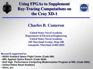
Using FPGAs to Supplement Ray-Tracing Computations on the Cray XD-1. Charles B. Cameron. United States Naval Academy Department of Electrical Engineering United States Naval Academy 105 Maryland Avenue, Stop 14B Annapolis, Maryland 21402-5025. Research supported by:

E N D
Using FPGAs to Supplement Ray-Tracing Computations on the Cray XD-1 Charles B. Cameron United States Naval Academy Department of Electrical Engineering United States Naval Academy 105 Maryland Avenue, Stop 14B Annapolis, Maryland 21402-5025 • Research supported by: • NASA Goddard Space Flight Center (Code 586) • NRL Applied Optics Branch (Code 5630) • DoD High Performance Computing Modernization Program at NRL (Code 5593) • United States Naval Academy • Xilinx, Inc.
Topics • Ray tracing • Conventional parallel processing • Modulo scheduling • Coordination of sequential and parallel processing • Expected Performance
Ray tracing • MODIS • Moderate-resolution Imaging Spectroradiometer • The Intersection Problem • Finding the Perpendicular • Refraction • Reflection
MODIS Optical System (Moderate-resolution Imaging Spectroradiometer)
MODIS Optical System • 485 pinholes • 400 rays per pinhole • 241 ´ 121 rays reflected from the diffuser • 5.66 ´ 109 rays
Ray Directed to a Surface • MODIS • Moderate-resolution Imaging Spectroradiometer • The Intersection Problem • Finding the Perpendicular • Refraction • Reflection • Coordinate Transformation
Calculate the Intercept Point • MODIS • Moderate-resolution Imaging Spectroradiometer • The Intersection Problem • Finding the Perpendicular • Refraction • Reflection • Coordinate Transformation
Find the Normal • MODIS • Moderate-resolution Imaging Spectroradiometer • The Intersection Problem • Finding the Perpendicular • Refraction • Reflection • Coordinate Transformation
Find the Refracted Ray • MODIS • Moderate-resolution Imaging Spectroradiometer • The Intersection Problem • Finding the Perpendicular • Refraction • Reflection • Coordinate Transformation
Find the Reflected Ray • MODIS • Moderate-resolution Imaging Spectroradiometer • The Intersection Problem • Finding the Perpendicular • Refraction • Reflection • Coordinate Transformation
Coordinate Transformation • MODIS • Moderate-resolution Imaging Spectroradiometer • The Intersection Problem • Finding the Perpendicular • Refraction • Reflection • Coordinate Transformation (Hard to visualize this!)
Topics • Ray tracing • Conventional parallel processing • Modulo scheduling • Coordination of sequential and parallel processing • Expected Performance
Performance (5.66 ´ 109 rays) * 99.998 % 5,857 % * Rate based on a linear regression of results obtained using a varying numbers of processors.
Topics • Ray tracing • Conventional parallel processing • Modulo scheduling • Coordination of sequential and parallel processing • Expected Performance
Operations Required as a Function of Surface, Aperture, and Interaction Types Not too many of these Lots of these
Quadratic Equation Latency Critical Path (Data-Flow Limit) 88 cycles
Modulo Scheduling:One Multiplier Equal to the Data-Flow Limit
Modulo Scheduling:Filling the Pipeline One collective computation
Modulo Scheduling:Filling the Pipeline Multipliers are 100 % utilized No schedule conflicts
Modulo Scheduling:Two Multipliers Two multipliers with two multiplications each
Modulo Scheduling:Two Multipliers One adder with two additions Two cycles Maximum efficiency
Modulo Scheduling:Two Multipliers Improved efficiency: Up from 25 %
Modulo Scheduling:Two Multipliers Less than the Data-Flow Limit
Modulo Scheduling:Two Multipliers Less than the Data-Flow Limit, but double the throughput.
Topics • Ray tracing • Conventional parallel processing • Modulo scheduling • Coordination of sequential and parallel processing • Expected Performance
Cray XD-1 • MPI (Message Passing Interface) • Master node • Reads file • Distributes file • Collates results
One Node of the Cray XD-1 • Open MP (Multi Processing) • 144 of 220 nodes have a Xilinx Virtex II Pro FPGA • Opteron processors • Sequential program • Depth first • FPGA • Pipelined hardware • Breadth first
Topics • Ray tracing • Conventional parallel processing • Modulo scheduling • Coordination of sequential and parallel processing • Expected Performance
Summary • Modulo scheduling produces 100 % efficiency of critical resources. • Sequential processors get a boost from supplemental FPGA processing. • Deep pipelines are efficient only if filled much of the time. • FPGAs beat ASICs only if they can take advantage of special problem knowledge. • Opteron uses 55 W. • Virtex II Pro FPGA uses 4 W to 45 W.
Equations • Intersection of a Ray with a Plane • Intersection of a Ray with a Sphere • Intersection of a Ray with a Conicoid • Finding the Perpendicular • Interaction of a Ray with an Optical Surface • Coordinate Transformations
Intersection of a Ray with a Plane Point in the plane Initial direction Final point Initial point Normal to the plane List of equations
Intersection of a Ray with a Sphere Initial direction Final point Initial point List of equations
Intersection of a Ray with a Conicoid Final point Initial point Initial direction List of equations