Regression Analysis in the Literature

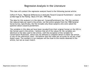
1. Regression Analysis in the Literature This class will conduct the regression analysis found in the following journal article: Clifton P. Flynn, "Regional Differences in Attitudes Toward Corporal Punishment." Journal of Marriage & the Family. 56(2):314-324. 1994 May. The data for this analysis is in the data set: CorporalPunishment.Sav. This file contains the reduced data set used in the article, not the entire sample from the 1988 General Social Survey. Specifically, the file includes only those subjects who were asked the question about corporal punishment. The variables in this data set have been recoded from their original format on the GSS to the format used in the article. I believe that all of the values for the variables are identical to the data used in the article, with the exception of the variable for Conservative Protestant, which was not defined in complete detail in either the article or any of the references cited. I do believe that the codes are accurate for all but a half dozen cases. The numbers in our analyses will be close to the results obtained in the article, but not an exact match. Regression Analysis in the Literature

2. Stage 1: Definition Of The Research Problem In the first stage, we state the research problem, specify the variables to be used in the analysis, and specify the method for conducting the analysis: standard multiple regression, hierarchical regression, or stepwise regression. Relationship to be Analyzed The question to be answered in the regression analyses is stated on page 316 of the article: to determine whether any regional differences in spanking attitudes remain after controlling for important social factors; and to assess whether the relationship between the control variables and attitudes toward corporal punishment is the same within each region. Regression Analysis in the Literature

3. Specifying the Dependent and Independent Variables The dependent variable for this study was attitude toward spanking (SPANKING). This variable was measured using the following item: "Do you strongly agree, agree, disagree, or strongly disagree that it is sometimes necessary to discipline a child with a good, hard spanking?" Responses were coded from 1 to 4, with 4 being "strongly agree," so that a higher score indicated a more favorable attitude toward corporal punishment. Region of the country served as the predictor independent variable (REGION) The analysis included eight control independent variables: • Income - measured using 20 income ranges, which were coded from lowest (1)--under $1,000--to highest (20)--$60,000 or over (INCOME86) • Age (AGE) • Number of children (CHILDS) • Years of schooling completed (EDUC) • Sex - coded as female and male (FEMALE) • Race - coded as blacks and nonblacks (BLACK) • Religion - coded as conservative Protestants versus compared to all other respondents. (CONSPROT) • Native residence - coded as rural natives and nonrural natives. A rural native was defined as one who resided in a community of fewer than 50,000 people both at age 16 and at the time of the survey. (RURALNAT) Regression Analysis in the Literature

4. Method for including independent variables: standard, hierarchical, stepwise While the structure of the question suggests a hierarchical regression, the author opts to do standard multiple regression. Both methods produce the same result, but the change in R² statistic is not available in standard multiple regression. Since we are replicating the analysis, we will do standard multiple regression. Regression Analysis in the Literature

5. Stage 2: Develop The Analysis Plan: Sample Size Issues In stage 2, we examine sample size and measurement issues. Missing data analysis To test for missing data, we run the SPSS script MissingDataCheck.SBS.  This script tallies the number of missing variables per case and the number of missing cases per variable.  It will filter out cases missing large numbers of variables, e.g. more than 50% of the variables included in the missing data check.  The script also creates a pattern variable and a correlation matrix of dichotomous missing/valid variables.  It does not do the t-tests or chi-square tests to compare missing and valid groupings on one variable to the pattern of values on other variables. Regression Analysis in the Literature

6. Run the MissingDataCheck Script Regression Analysis in the Literature

7. Complete the 'Check for Missing Data' Dialog Box Regression Analysis in the Literature

8. The Number of Missing Cases for Each Variable In the frequency table that lists each variable and the number of missing and valid cases, we see that the variable with the largest number of missing cases is Total Family Income, with 80 cases. The number of missing cases for the other variables is negligible. Regression Analysis in the Literature

9. Patterns of Missing Variables Only one case had two missing variables, Age and Total Family Income. The most prevalent pattern concerns the Total Family Income variable, which we had already detected. There does not appear to be any pattern of missing variables about which we should be concerned. Regression Analysis in the Literature

10. The Correlation Matrix of Valid/Missing Dichotomous Variables In the segment of the matrix shown below, there are not any correlations about 0.40. If we inspect the remainder of the matrix in the output, we will not find any moderate correlations. The correlation matrix does not support the presence of a missing data process. Regression Analysis in the Literature

11. Recoding for Missing Data The authors of the article opt to do substitution for the missing cases.  For the metric variables we can specify Mean Substitution on the Regression command to solve this problem.  For the nonmetric variables, the authors employ modal substitution, which I take to mean substituting the largest category on each of the nonmetric variables that have missing data (Conservative Protestant and Rural Native).  We can accomplish this modal substitution by running the following syntax commands: RECODE consprot ruralnat  (MISSING=0). EXECUTE. Regression Analysis in the Literature

12. Power to Detect Relationships The table on page 165 of the text indicates that our sample size will show statistical significance for very small R² values, e.g. 2%, even at the conservative alpha value of 0.01. I extracted this from the sample size row of 1000 and the number of independent variables of 10. Minimum Sample Size Requirement: 15-20 Cases Per Independent Variable A sample size of 978 cases and 11 independent variables (the eight control variables plus the three dummy coded variables for region) produces a case to variable ration of 89 to 1, far in excess of the guideline of 15-20 cases per independent variable. Regression Analysis in the Literature

13. Stage 2: Develop The Analysis Plan: Measurement Issues In this part of stage 2, we examine measurement issues. Incorporating Nonmetric Data with Dummy Variables The nonmetric variables for female, black, conservative protestant, and rural have already been dummy-coded. The original region variable contains nine categories. To see the codes for these nine categories, select the Variables... command from the Utilities menu and select the region variable. The division for regions in the article uses four categories:  Northeast, West, Midwest, and South. The dummy coding for four regions would normally require the creation of three new variables. However, we created the full set of four to support the individual regressions for each region.  These variables have already been added to the data set. Regression Analysis in the Literature

14. Incorporating Nonmetric Data with Dummy Variables The nonmetric variables for female, black, conservative protestant, and rural have already been dummy-coded. The original region variable contains nine categories. To see the codes for these nine categories, select the Variables... command from the Utilities menu and select the region variable. The division for regions in the article uses four categories:  Northeast, West, Midwest, and South. The dummy coding for four regions would normally require the creation of three new variables. However, we created the full set of four to support the individual regressions for each region.  These variables have already been added to the data set. Representing Curvilinear Effects with Polynomials We do not have any evidence of curvilinear effects at this point in the analysis. Representing Interaction or Moderator Effects We do not have any evidence at this point in the analysis that we should add interaction or moderator variables. Regression Analysis in the Literature

15. Stage 3: Evaluate Underlying Assumptions In this stage, we verify that all of the independent variables are metric or dummy-coded, and test for normality of the metric variables, linearity of the relationships between the dependent and the independent variables, and test for homogeneity of variance for the nonmetric independent variables. Metric Dependent Variable and Metric or Dummy-coded Independent Variables All of the variables in the analysis are metric or have already been dummy coded. Regression Analysis in the Literature

16. Normality of metric variables The null hypothesis in the K-S Lilliefors test of normality is that the data for the variable is normally distributed. The desirable outcome for this test is to fail to reject the null hypothesis.  When the probability value in the Sig. column is less than 0.05, we conclude that the variable is not normally distributed.  If a variable is not normally distributed, we can try three transformations (logarithmic, square root, and inverse) to see if we can induce the distribution of cases fit a normal distribution.  If one or more of the transformations induces normality, we have the option of substituting the transformed variable in the analysis to see if it improves the strength of the relationship. To test for normality, we will run the NormalityAssumptionAndTransformations.SBS script and test the metric variables:  CHILDS  'NUMBER OF CHILDREN', AGE  'AGE OF RESPONDENT', EDUC  'HIGHEST YEAR OF SCHOOL COMPLETED', INCOME86  'TOTAL FAMILY INCOME', and SPANKING  'FAVOR SPANKING TO DISCIPLINE CHILD'. Regression Analysis in the Literature

17. Run the 'NormalityAssumptionAndTransformations' Script Regression Analysis in the Literature

18. Complete the 'Test for Assumption of Normality' Dialog Box Regression Analysis in the Literature

19. Output for the Tests of Normality Explore the output for the tests of normality to confirm that all the metric variables failed the normality test and, furthermore, none of the transformations produced a variable that was normally distributed. Regression Analysis in the Literature

20. Linearity between metric independent variables and dependent variable Another script, 'LinearityAssumptionAndTransformations' tests for linearity of relationships between the dependent variable and each of the independent variables.  Since there is no simple score that indicates whether or not a relationship is linear or nonlinear, a scatterplot matrix is created for the dependent variable, the independent variable, and transformations of the independent variable.  The user can visually inspect the scatterplot matrix for evidence of nonlinearity.  If nonlinearity is evident, but not corrected by a transformation of the independent variable, transformation of the dependent variable is available.  More detailed information is available by requesting a correlation matrix for the variables included in the scatterplot matrix.  If the scatterplot matrix does not provide sufficient detail, individual scatterplots overlaid with fit lines can be requested. When we run the script as described below, we do not find any nonlinear relationships between the dependent variables and the metric independent variables. Regression Analysis in the Literature

21. Run the 'LinearityAssumptionAndTransformations' Script Regression Analysis in the Literature

22. Complete the 'Check for Linear Relationships' Dialog Box Regression Analysis in the Literature

23. The Scatterplot Matrix The scatterplot matrices produced for this analysis have a different look because the dependent variable contains only four discrete categories, so all of the values will line up in four vertical columns. The relationship can still be evaluated for linearity by determining whether or not the fit line crosses the vertical columns in an ascending or descending pattern from left to right, or whether the bars in the center are higher, or lower, than the surrounding bars. Regression Analysis in the Literature

24. Constant variance across categories of nonmetric independent variables Another script, 'HomoscedasticityAssumptionAndTransformations' tests for homogeneity of variance across groups designated by nonmetric independent variables.  The script uses the One-Way ANOVA procedure to produce a Levene test of the homogeneity of variance. The null hypothesis of the Levene test is that the variance of all groups of the independent variable are equal.  If the Sig value associated with the test is greater than the alpha level, we fail to reject the null hypothesis and conclude that the variance for all groups is equivalent.  If the Sig value associated with the test is less than the alpha level, we reject the null hypothesis and conclude that the variance of at least one group is different.  If we fail the homogeneity of variance test, we can attempt to correct the problem by applying the transformations for normality to the dependent variable specified in the test.  The script computes the transformations and applies the Levene test to the transformed variables.  If one of the transformed variables corrects the problem, we can consider substituting it for the original form of the variable. Regression Analysis in the Literature

25. Run the 'HomoscedasticityAssumptionAndTransformations' Script Regression Analysis in the Literature

26. Complete the 'Test for Assumption of Homogeneity of Variance' Dialog Box Regression Analysis in the Literature

27. Output for theTest of Homogeneity of Variances The output for the tests of homoegeneity of variances indicates that the variables FEMALE  'Female' and NORTHEAS  'Northeast Region' do not pass the Levene test. An inverse transformation of the dependent variable would correct the problem for the female variable, while a log or square root transformation corrects the homogeneity problem for the northeast variable.  Since no transformation would solve both problems and since we did not find a transformation that corrected the normality problem for the spanking variable, we will not consider a transformation any further. Regression Analysis in the Literature

28. Stage 4: Compute the Statistics And Test Model Fit: Computations In this stage, we compute the actual statistics to be used in the analysis. Regression requires that we specify a variable selection method. The article specifies standard multiple regression. Compute the Regression Model The first task in this stage is to request the initial regression model and all of the statistical output we require for the analysis. Regression Analysis in the Literature

29. Request the Regression Analysis Regression Analysis in the Literature

30. Specify the Dependent and Independent Variables and the Variable Selection Method Regression Analysis in the Literature

31. Specify the Statistics Options Regression Analysis in the Literature

32. Complete the Linear Regression Statistics Dialog Regression Analysis in the Literature

33. Specify the Plots to Include in the Output Regression Analysis in the Literature

34. Complete the Linear Regression Plots dialog box Regression Analysis in the Literature

35. Specify Diagnostic Statistics to Save to the Data Set Regression Analysis in the Literature

36. Complete the Linear Regression Save dialog box. Regression Analysis in the Literature

37. Specify the Mean Substitution Option Regression Analysis in the Literature

38. Complete the Linear Regression: Options dialog box Regression Analysis in the Literature

39. Stage 4: Compute the Statistics And Test Model Fit: Model Fit In this stage, we examine the relationships between our independent variables and the dependent variable.  First, we look at the F test for R Square which is associated with the overall relationship between the dependent variable and the set of independent variables.  The F statistic tests the hypothesis that there is no relationship between the dependent variable and the set of independent variables, i.e. the null hypothesis is: R² = 0.  If we cannot reject this null hypothesis, then our analysis is concluded; there is no relationship between the dependent variable and the independent variables that we can interpret. If we reject the null hypothesis and conclude that there is a relationship between the dependent variable and the set of independent variables, then we examine the table of coefficients to identify which independent variables have a statistically significant individual relationship with the dependent variable.  For each independent variable in the analysis, a t-test is computed that the slope of the regression line (B) between the independent variable and the dependent variable is not zero.  The null hypothesis is that the slope is zero, i.e. B = 0, implying that the independent variable has no impact or relationship on scores on the dependent variable.  This part of the analysis is most important in standard multiple regression where we enter all of the independent variables into the regression at one time, and hierarchical multiple regression where we specify the order of entry of independent variables than it is in stepwise multiple regression where the computer picks the order of entry and stops adding variables when some statistical limit is reached.  In stepwise regression, we would expect all of the individual variables that passed the statistical entry for entry to have a significant individual relationship with the dependent variable. Regression Analysis in the Literature

40. Stage 4: Compute the Statistics And Test Model Fit: Model Fit When we are determining which independent variables have a significant relationship with the dependent variable, we often are interested in the question of the relative importance of the predictor variables to predicting the dependent variable.  To answer this question, we will examine the Beta coefficients, or standardized version of the coefficients of the individual independent variables. Regression Analysis in the Literature

41. 1. Significance Test of the Coefficient of Determination R Square In the ANOVA table, we see that R² of 0.111 is associated with a statistically significant relationship (sig < 0.0001) between the dependent variable and the independent variables. We reject the null hypothesis that R² is zero and conclude that there is a relationship between the independent variables and the dependent variable. Regression Analysis in the Literature

42. 2. Significance Test of Individual Regression Coefficients The interpretation of the coefficients would be identical to that found in the article in the first column on page 320. Looking at the Sig column for the tests of individual coefficients, we see that number of children, years of education, conservative Protestant, ethnicity, rural native, and Northeast region all have significant individual relationships with the dependent variable of favoring spanking. (Note that the numbers in our table follow the same general pattern as the article, but are not identical.) Regression Analysis in the Literature

43. Stage 4: Compute the Statistics And Test Model Fit: Meeting Assumptions Using output from the regression analysis to examine the conformity of the regression analysis to the regression assumptions is often referred to as "Residual Analysis" because if focuses on the component of the variance which our regression model cannot explain.  Using the regression equation, we can estimate the value of the dependent variable for each case in our sample.  This estimate will differ from the actual score for each case by an amount referred to as the residual.  Residuals are a measure of unexplained variance or error that remains in the dependent variable that cannot be explained or predicted by the regression equation. Regression Analysis in the Literature

44. Linearity and Constant Variance for the Dependent Variable - Residual Plot The residual plot shows the pattern that is associated with a discrete dependent variable, i.e. if there are four possible values for the dependent variable, the residuals will fall in bands associated with these values. If the residuals are randomly distributed, the bands will tend to fill the graphic space both vertically and horizontally. The lack of data points in the upper righthand corner and lower lefthand corner are a result of the restricted range of the possible values of the dependent variable and are not indicative of a problem with underlying assumptions. I cannot identify any violation of homoscedasticity or nonlinear trend in the plot of residuals. The tendency to have a larger number of points in the left half of the chart is associated with the normality problem of the dependent variable which we could not correct. Regression Analysis in the Literature

45. Normal Distribution of Residuals - Normality Plot of Residuals To check for meeting the assumption that the residuals or error terms are normally distributed, we look at the Normal p-p plot of Regression Standardized Residual as shown to the right. Our criteria is the degree to which the plot for the actual values coincides with the green line of expected values. For this problem, the plot of residuals fits the expected pattern well enough to support a conclusion that the residuals are normally distributed. If a more exact computation is desired, we instruct SPSS to save the residuals in our data file and do a test of normality on the residual values using the Explore command. Regression Analysis in the Literature

46. Linearity of Independent Variables - Partial Plots To verify the assumption of linearity for the metric independent variables, we examine the partial regression plots. The partial plots for the numeric variables, Age, Number of Children, Education level, and Income in this analysis do not show any nonlinear patterns. All show a weak linear relationship, like the partial plot for number of children shown below. We ignore the partial plots for the dummy-coded variables as extraneous output since linearity is not an expectation for nonmetric variables. Regression Analysis in the Literature

47. Independence of Residuals - Durbin-Watson Statistic The next assumption is that the residuals are not correlated serially from one observation to the next. This means the size of the residual for one case has no impact on the size of the residual for the next case. While this is particularly a problem for time-series data, SPSS provides a simple statistical measure for serial correlation for all regression problems. The Durbin-Watson Statistic is used to test for the presence of serial correlation among the residuals. Unfortunately, SPSS does not print the probability for accepting or rejecting the presence of serial correlation, though probability tables for the statistic are available in other texts. The value of the Durbin-Watson statistic ranges from 0 to 4. As a general rule of thumb, the residuals are uncorrelated is the Durbin-Watson statistic is approximately 2. A value close to 0 indicates strong positive correlation, while a value of 4 indicates strong negative correlation. For our problem, the value of Durbin-Waston is 1.909, approximately equal to 2, indicating no serial correlation. Regression Analysis in the Literature

48. Identifying Dependent Variable Outliers - Casewise Plot of Standardized Residuals As shown in the following table of Residual Statistics, all standardized residuals (Std. Residual) fell within +/- 3 standard deviations. We do not have cases where the value of the dependent variable indicates an outlier Regression Analysis in the Literature

49. Identifying Independent Variable Outliers - Mahalanobis Distance To identify only the most extreme outliers, the level of significance used is set to 0.001.  The critical value of Mahalanobis Distance for 11 independent variables is 30.264.  The table of residual statistics shows that the maximum Mahalanobis distance found for any case is 30.831, which is larger than the critical value.  While we should, perhaps. re-run the analysis excluding this case, we will skip this test for the pragmatic reason that 1 case out of 978 with a problematic distance score will not affect the analysis. Regression Analysis in the Literature

50. Identifying Influential Cases - Cook's Distance Cook's distance identifies cases that are influential or have a large effect on the regression solution and may be distorting the solution for the remaining cases in the analysis.  While we cannot associate a probability with Cook's distance, we can identify problematic cases that have a score larger than the criteria computed using the formula: 4/(n - k - 1), where n is the number of cases in the analysis and k is the number of independent variables.  For this problem which has 978 subjects and 11 independent variables, the formula equates to: 4 / (978 - 11 - 1) = 0.004.  To identify the influential cases with large Cook's distances, we sort the data set by the Cook's distance variable, 'coo_1' that SPSS created in the data set. Regression Analysis in the Literature