Download
1 / 128
1.75k likes | 3.34k Views
Mathematical Foundation of Photogrammetry (part of EE5358). Dr. Venkat Devarajan Ms. Kriti Chauhan. Photogrammetry. photo = "picture“, grammetry = "measurement“, therefore photogrammetry = “photo-measurement”.

E N D
Mathematical Foundation of Photogrammetry (part of EE5358) Dr. Venkat Devarajan Ms. Kriti Chauhan
Photogrammetry photo = "picture“, grammetry = "measurement“, therefore photogrammetry = “photo-measurement” Photogrammetry is the science or art of obtaining reliable measurements by means of photographs. Formal Definition: Photogrammetry is the art, science and technology of obtaining reliable information about physical objects and the environment, through processes of recording, measuring, and interpreting photographic images and patterns of recorded radiant electromagnetic energy and other phenomena. - As given by the American Society for Photogrammetry and Remote Sensing (ASPRS) Virtual Environment Lab, UTA Chapter 1
Distinct Areas Interpretative Photogrammetry Metric Photogrammetry Deals in recognizing and identifying objects and judging their significance through careful and systematic analysis. • making precise measurements from photos determine the relative locations of points. • finding distances, angles, areas, volumes, elevations, and sizes and shapes of objects. • Most common applications: • preparation of planimetric and topographic maps • production of digital orthophotos • Military intelligence such as targeting Photographic Interpretation Remote Sensing (Includes use of multispectral cameras, infrared cameras, thermal scanners, etc.) Virtual Environment Lab, UTA Chapter 1
Uses of Photogrammetry • Products of photogrammetry: • Topographic maps: detailed and accurate graphic representation of cultural and natural features on the ground. • Orthophotos: Aerial photograph modified so that its scale is uniform throughout. • Digital Elevation Maps (DEMs): an array of points in an area that have X, Y and Z coordinates determined. • Current Applications: • Land surveying • Highway engineering • Preparation of tax maps, soil maps, forest maps, geologic maps, maps for city and regional planning and zoning • Traffic management and traffic accident investigations • Military – digital mosaic, mission planning, rehearsal, targeting etc. Virtual Environment Lab, UTA Chapter 1
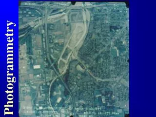
Types of photographs Aerial Terrestrial Oblique Vertical Low oblique (does not include horizon) Truly Vertical High oblique (includes horizon) Tilted (1deg< angle < 3deg) Virtual Environment Lab, UTA Chapter 1
Of all these type of photographs, vertical and low oblique aerial photographs are of most interest to us as they are the ones most extensively used for mapping purposes… Virtual Environment Lab, UTA
Aerial Photography Vertical aerial photographs are taken along parallel passes called flight strips. Successive photographs along a flight strip overlap is called end lap – 60% Area of common coverage called stereoscopic overlap area. Overlapping photos called a stereopair. Virtual Environment Lab, UTA Chapter 1
Aerial Photography Position of camera at each exposure is called the exposure station. Altitude of the camera at exposure time is called the flying height. Lateral overlapping of adjacent flight strips is called a side lap (usually 30%). Photographs of 2 or more sidelapping strips used to cover an area is referred to as a block of photos. Virtual Environment Lab, UTA Chapter 1
Now, lets examine the acquisition devices for these photographs… Virtual Environment Lab, UTA
Camera / Imaging Devices The general term “imaging devices” is used to describe instruments used for primary photogrammetric data acquisition. • Types of imaging devices (based on how the image is formed): • Frame sensors/cameras: acquire entire image simultaneously • Strip cameras, Linear array sensors or Pushbroom scanners: sense only a linear projection (strip) of the field of view at a given time and require device to sweep across the “gaming” area to get a 2D image • Flying spot scanners or mechanical scanners: detect only a small spot at a time, require movement in two directions (sweep and scan) to form 2D image. Virtual Environment Lab, UTA Chapter 3
Aerial Mapping Camera Aerial mapping cameras are the traditional imaging devices used in traditional photogrammetry. Virtual Environment Lab, UTA Chapter 3
Lets examine terms and characteristics associated with a camera, parameters of a camera, and how to determine them… Virtual Environment Lab, UTA
Focal Plane of Aerial Camera The focal plane of an aerial camera is the plane in which all incident light rays are brought to focus. Focal plane is set as exactly as possible at a distance equal to the focal length behind the rear nodal point of the camera lens. In practice, the film emulsion rests on the focal plane. Rear nodal point: The emergent nodal point of a thick combination lens. (N’ in the figure) Note: Principal point is a 2D point on the image plane. It is the intersection of optical axis and image plane. Virtual Environment Lab, UTA Chapter 3
Fiducials in Aerial Camera Fiducials are 2D control points whose xy coordinates are precisely and accurately determined as a part of camera calibration. Fiducial marks are situated in the middle of the sides of the focal plane opening or in its corners, or in both locations. They provide coordinate reference for principal point and image points. Also allow for correction of film distortion (shrinkage and expansion) since each photograph contains images of these stable control points. Lines joining opposite fiducials intersect at a point called the indicated principal point. Aerial cameras are carefully manufactured so that this occurs very close to the true principal point. True principal point: Point in the focal plane where a line from the rear nodal point of the camera lens, perpendicular to the focal plane, intersects the focal plane. Virtual Environment Lab, UTA Chapter 3
Elements of Interior Orientation • Elements of interior orientation are the parameters needed to determine accurate spatial information from photographs. These are as follows: • Calibrated focal length (CFL), the focal length that produces an overall mean distribution of lens distortion. • Symmetric radial lens distortion, the symmetric component of distortion that occurs along radial lines from the principal point. Although negligible, theoretically always present. • Decentering lens distortion, distortion that remains after compensating for symmetric radial lens distortion. Components: asymmetric radial and tangential lens distortion. • Principal point location, specified by coordinates of a principal point given wrt x and y coordinates of the fiducial marks. • Fiducial mark coordinates: x and y coordinates which provide the 2D positional reference for the principal point as well as images on the photograph. • The elements of interior orientation are determined through camera calibration. Virtual Environment Lab, UTA Chapter 3
Other Camera Characteristics • Other camera characteristics that are often of significance are: • Resolution for various distances from the principal point (highest near the center, lowest at corners of photo) • Focal plane flatness: deviation of platen from a true plane. Measured by a special gauge, generally not more than 0.01mm. • Shutter efficiency: ability of shutter to open instantaneously, remain open for the specified exposure duration, and close instantaneously. Virtual Environment Lab, UTA Chapter 3
Camera Calibration: General Approach • Step 1) Photograph an array of targets whose relative positions are accurately known. • Step 2) Determine elements of interior orientation – • make precise measurements of target images • compare actual image locations to positions they should have occupied had the camera produced a perfect perspective view. • This is the approach followed in most methods. Virtual Environment Lab, UTA Chapter 3
After determining interior camera parameters, we consider measurements of image points from images… Virtual Environment Lab, UTA
Photogrammetric Scanners Photogrammetric scanners are the devices used to convert the content of photographs from analog form (a continuous-tone image) to digital form (an array of pixels with their gray levels quantified by numerical values). Coordinate measurement on the acquired digital image can be done either manually, or through automated image-processing algorithms. Requirements: sufficient geometric and radiometric resolution, and high geometric accuracy. Geometric/spatial resolution indicates pixel size of resultant image. Smaller the pixel size, greater the detail that can be detected in the image. For high quality photogrammetric scanners, min pixel size is on the order of 5 to 15µm Radiometric resolution indicates the number of quantization levels. Min should be 256 levels (8 bit); most scanners capable of 1024 levels (10 bit) or higher. Geometric quality indicates the positional accuracy of pixels in the resultant image. For high quality scanners, it is around 2 to 3 µm. Virtual Environment Lab, UTA Chapter 4
Sources of Error in Photo Coordinates • The following are some of the sources of error that can distort the true photo coordinates: • Film distortions due to shrinkage, expansion and lack of flatness • Failure of fiducial axes to intersect at the principal point • Lens distortions • Atmospheric refraction distortions • Earth curvature distortion • Operator error in measurements • Error made by automated correlation techniques Virtual Environment Lab, UTA Chapter 4
Now that we have covered the basics of image acquisition and measurement, we turn to analytical photogrammetry… Virtual Environment Lab, UTA
Analytical Photogrammetry • Definition: Analytical photogrammetry is the term used to describe the rigorous mathematical calculation of coordinates of points in object space based upon camera parameters, measured photo coordinates and ground control. • Features of Analytical photogrammetry: • rigorously accounts for any tilts • generally involves solution of large, complex systems of redundant equations by the method of least squares • forms the basis of many modern hardware and software system including stereoplotters, digital terrain model generation, orthophoto production, digital photo rectification and aerotriangulation. Virtual Environment Lab, UTA Chapter 11
Image Measurement Considerations • Before using the x and y photo coordinate pair, the following conditions should be considered: • Coordinates (usually in mm) are relative to the principal point - the origin. • Analytical photogrammetry is based on assumptions such as “light rays travel in straight lines” and “the focal plane of a frame camera is flat”. Thus, coordinate refinements may be required to compensate for the sources of errors, that violate these assumptions. • Measurements must be ensured to have high accuracy. • While making measurements of image coordinates of common points that appear in more than one photograph, each object point must be precisely identified between photos so that the measurements are consistent. • Object space coordinates is based on a 3D cartesian system. Virtual Environment Lab, UTA Chapter 11
Now, we come to the most fundamental and useful relationship in analytical photogrammetry, the collinearity condition… Virtual Environment Lab, UTA
Collinearity Condition The collinearity condition is illustrated in the figure below. The exposure station of a photograph, an object point and its photo image all lie along a straight line. Based on this condition we can develop complex mathematical relationships. Virtual Environment Lab, UTA Appendix D
Collinearity Condition Equations Let: Coordinates of exposure station be XL, YL, ZL wrt object (ground) coordinate system XYZ Coordinates of object point A be XA, YA, ZA wrt ground coordinate system XYZ Coordinates of image point a of object point A be xa, ya, za wrt xy photo coordinate system (of which the principal point o is the origin; correction compensation for it is applied later) Coordinates of image point a be xa’, ya’, za’ in a rotated image plane x’y’z’ which is parallel to the object coordinate system Transformation of (xa’, ya’, za’) to (xa, ya, za) is accomplished using rotation equations, which we derive next. Virtual Environment Lab, UTA Appendix D
Rotation Equations Omega rotation about x’ axis: New coordinates (x1,y1,z1) of a point (x’,y’,z’) after rotation of the original coordinate reference frame about the x axis by angle ω are given by: x1 = x’ y1 = y’ cos ω + z’ sin ω z1 = -y’sin ω + z’ cos ω Similarly, we obtain equations for phi rotation about y axis: x2 = -z1sin Ф + x1 cos Ф y2 = y1 z2 = z1 cos Ф + x1 sin Ф And equations for kappa rotation about z axis: x = x2 cos қ + y2 sin қ y = -x2 sin қ + y2 cos қ z = z2 Virtual Environment Lab, UTA Appendix C
Final Rotation Equations We substitute the equations at each stage to get the following: x = m11 x’ + m12 y’ + m13 z’ y = m21 x’ + m22 y’ + m23 z’ z = m31 x’ + m32 y’ + m33 z’ Where m’s are function of rotation angles ω,Ф and қ In matrix form: X = M X’ where • Properties of rotation matrix M: • Sum of squares of the 3 direction cosines (elements of M) in any row or column is unity. • M is orthogonal, i.e. M-1 = MT Virtual Environment Lab, UTA Appendix C
Coming back to the collinearity condition… Virtual Environment Lab, UTA
Collinearity Equations Using property of similar triangles: Substitute this into rotation formula: Now, factor out za’/(ZA-ZL), divide xa, ya by za add corrections for offset of principal point (xo,yo) and equate za=-f, to get: Virtual Environment Lab, UTA Appendix D
Review of Collinearity Equations Collinearity equations: • Collinearity equations: • are nonlinear and • involve 9 unknowns: • omega, phi, kappa inherent in the m’s • Object coordinates (XA, YA, ZA ) • Exposure station coordinates (XL, YL, ZL ) Where, xa, ya are the photo coordinates of image point a XA, YA, ZA are object space coordinates of object/ground point A XL, YL, ZL are object space coordinates of exposure station location f is the camera focal length xo, yo are the offsets of the principal point coordinates m’s are functions of rotation angles omega, phi, kappa (as derived earlier) Virtual Environment Lab, UTA Ch. 11 & App D
Now that we know about the collinearity condition, lets see where we need to apply it. First, we need to know what it is that we need to find… Virtual Environment Lab, UTA
Elements of Exterior Orientation • As already mentioned, the collinearity conditions involve 9 unknowns: • Exposure station attitude (omega, phi, kappa), • Exposure station coordinates (XL, YL, ZL ), and • Object point coordinates (XA, YA, ZA). • Of these, we first need to compute the position and attitude of the exposure station, also known as the elements of exterior orientation. • Thus the 6 elements of exterior orientation are: • spatial position (XL, YL, ZL) of the camera and • angular orientation (omega, phi, kappa) of the camera • All methods to determine elements of exterior orientation of a single tilted photograph, require: • photographic images of at least three control points whose X, Y and Z ground coordinates are known, and • calibrated focal length of the camera. Virtual Environment Lab, UTA Chapter 10
As an aside, from earlier discussion: Elements of Interior Orientation • Elements of interior orientation which can be determined through camera calibration are as follows: • Calibrated focal length (CFL), the focal length that produces an overall mean distribution of lens distortion. Better termed calibrated principal distance since it represents the distance from the rear nodal point of the lens to the principal point of the photograph, which is set as close to optical focal length of the lens as possible. • Principal point location, specified by coordinates of a principal point given wrt x and y coordinates of the fiducial marks. • Fiducial mark coordinates: x and y coordinates of the fiducial marks which provide the 2D positional reference for the principal point as well as images on the photograph. • Symmetric radial lens distortion, the symmetric component of distortion that occurs along radial lines from the principal point. Although negligible, theoretically always present. • Decentering lens distortion, distortion that remains after compensating for symmetric radial lens distortion. Components: asymmetric radial and tangential lens distortion. Virtual Environment Lab, UTA Chapter 3
Next, we look at space resection which is used for determining the camera station coordinates from a single, vertical/low oblique aerial photograph… Virtual Environment Lab, UTA
Space Resection By Collinearity • Space resection by collinearity involves formulating the “collinearity equations” for a number of control points whose X, Y, and Z ground coordinates are known and whose images appear in the vertical/tilted photo. • The equations are then solved for the six unknown elements of exterior orientation that appear in them. • 2 equations are formed for each control point • 3 control points (min) give 6 equations: solution is unique, while 4 or more control points (more than 6 equations) allows a least squares solution (residual terms will exist) • Initial approximations are required for the unknown orientation parameters, since the collinearity equations are nonlinear, and have been linearized using Taylor’s theorem. Virtual Environment Lab, UTA Chapter 10 & 11
Coplanarity Condition A similar condition to the collinearity condition, is coplanarity, which is the condition that the two exposure stations of a stereopair, any object point and its corresponding image points on the two photos, all lie in a common plane. Like collinearity equations, the coplanarity equation is nonlinear and must be linearized by using Taylor’s theorem. Linearization of the coplanarity equation is somewhat more difficult than that of the collinearity equations. But, coplanarity is not used nearly as extensively as collinearity in analytical photogrammetry. Space resection by collinearity is the only method still commonly used to determine the elements of exterior orientation. Virtual Environment Lab, UTA
Initial Approximationsfor Space Resection • We need initial approximations for all six exterior orientation parameters. • Omega and Phi angles: For the typical case of near-vertical photography, initial values of omega and phi can be taken as zeros. • H: • Altimeter reading for rough calculations • Compute ZL (height H about datum plane) using ground line of known length appearing on the photograph • To compute H, only 2 control points are required, rest are redundant. Approximation can be improved by averaging several values of H. Virtual Environment Lab, UTA Chapter 11 & 6
Calculating Flying Height (H) Flying height H can be calculated using a ground line of known length that appears on the photograph. Ground line should be on fairly level terrain as difference in elevation of endpoints results in error in computed flying height. Accurate results can be obtained despite this though, if the images of the end points are approximately equidistant from the principal point of the photograph and on a line through the principal point. H can be calculated using equations for scale of a photograph: S = ab/AB = f/H (scale of photograph over flat terrain) Or S = f/(H-h) (scale of photograph at any point whose elevation above datum is h) Virtual Environment Lab, UTA Chapter 6
As an explanation of the equations from which H is calculated: Photographic Scale • S = ab/AB = f/H • SAB = ab/AB = La/LA = Lo/LO = f/(H-h) • where • S is scale of vertical photograph over a flat terrain • SAB is scale of vertical photograph over variable terrain • ab is distance between images of points A and B on the photograph • AB is actual distance between points A and B • f is focal length • La is distance between exposure station L & image a of point A on the photo positive • LA is distance between exposure station L and point A • Lo = f is the distance from L to principal point on the photograph • LO = H-h is the distance from L to projection of o onto the horizontal plane containing point A with h being height of point A from the datum plane • Note: For vertical photographs taken over variable terrain, there are an infinite number of different scales. Virtual Environment Lab, UTA Chapter 6
Initial Approx. for XL, YL and k • x’ and y’ ground coordinates of any point can be obtained by simply multiplying x and y photo coordinates by the inverse of photo scale at that point. • This requires knowing • f, H and • elevation of the object point Z or h. • A 2D conformal coordinate transformation (comprising rotation and translation) can then be performed, which relates these ground coordinates computed from the vertical photo equations to the control values: • X = a.x’ – b.y’ + TX; Y = a.y’ + b.x’ + TY • We know (x,y) and (x’,y’) for n sets are known giving us 2n equations. • The 4 unknown transformation parameters (a, b, TX, TY) can therefore be calculated by least squares. So essentially we are running the resection equations in a diluted mode with initial values of as many parameters as we can find, to calculate the initial parameters of those that cannot be easily estimated. • TX and TY are used as initial approximation for XL and YL, resp. • Rotation angle θ = tan-1(b/a) is used as approximation for κ (kappa). Virtual Environment Lab, UTA Chapter 11
Space Resection by Collinearity: Summary (To determine the 6 elements of exterior orientation using collinearity condition) • Summary of steps: • Calculate H (ZL) • Compute ground coordinates from assumed vertical photo for the control points. • Compute 2D conformal coordinate transformation parameters by a least squares solution using the control points (whose coordinates are known in both photo coordinate system and the ground control cood sys) • Form linearized observation equations • Form and solve normal equations. • Add corrections and iterate till corrections become negligible. • Summary of Initializations: • Omega, Phi -> zero, zero • Kappa -> Theta • XL, YL -> TX, TY • ZL ->flying height H Virtual Environment Lab, UTA Chapter 11
If space resection is used to determine the elements of exterior orientation for both photos of a stereopair, then object point coordinates for points that lie in the stereo overlap area can be calculated by the procedure known as space intersection… Virtual Environment Lab, UTA
Space Intersection By Collinearity Use: To determine object point coordinates for points that lie in the stereo overlap area of two photographs that make up a stereopair. Principle: Corresponding rays to the same object point from two photos of a stereopair must intersect at the point. For a ground point A: Collinearity equations are written for image point a1 of the left photo (of the stereopair), and for image point a2 of the right photo, giving 4 equations. The only unknowns are XA, YA and ZA. Since equations have been linearized using Taylor’s theorem, initial approximations are required for each point whose object space coordinates are to be computed. Initial approximations are determined using the parallax equations. Virtual Environment Lab, UTA Chapter 11
Parallax Equations • Parallax Equations: • pa = xa – x’a • hA = H – B.f/pa • XA = B.xa/pa • YA = B.ya/pa • where • hA is the elevation of point A above datum • H is the flying height above datum • B is the air base (distance between the exposure stations) • f is the focal length of the camera • pa is the parallax of point A • XA and YA are ground coordinates of point A in the coordinate system with origin at the datum point P of the Lpho, X axis is in same vertical plane as x and x’ flight axes and Y axis passes through the datum point of the Lpho and is perpendicular to the X axis • xa and ya are the photo coordinates of point a measured wrt the flight line axes on the left photo Virtual Environment Lab, UTA Chapter 8
Applying Parallax Equations to Space Intersection For applying parallax equations, H and B have to be determined: Since X, Y, Z coordinates for both exposure stations are known, H is taken as average of ZL1 and ZL2 and B = [ (XL2-XL1)2 + (YL2-YL1)2 ]1/2 The resulting coordinates from the parallax equations are in the arbitrary ground coordinate system. To convert them to, for instance WGS84, a conformal coordinate transformation is used. Virtual Environment Lab, UTA Chapter 11
Now that we know how to determine object space coordinates of a common point in a stereopair, we can examine the overall procedure for all the points in the stereopair... Virtual Environment Lab, UTA
Analytical Stereomodel • Aerial photographs for most applications are taken so that adjacent photos overlap by more than 50%. Two adjacent photographs that overlap in this manner form a stereopair. • Object points that appear in the overlap area of a stereopair constitute a stereomodel. • The mathematical calculation of 3D ground coordinates of points in the stereomodel by analytical photogrammetric techniques forms an analytical stereomodel. • The process of forming an analytical stereomodel involves 3 primary steps: • Interior orientation (also called “photo coordinate refinement”): Mathematically recreates the geometry that existed in the camera when a particular photograph was exposed. • Relative (exterior) orientation: Determines the relative angular attitude and positional displacement between the photographs that existed when the photos were taken. • Absolute (exterior) orientation: Determines the absolute angular attitude and positions of both photographs. • After these three steps are achieved, points in the analytical stereomodel will have object coordinates in the ground coordinate system. Virtual Environment Lab, UTA Chapter 11
Analytical Relative Orientation Analytical relative orientation involves defining (assuming) certain elements of exterior orientation and calculating the remaining ones. Initialization: If the parameters are set to the values mentioned (i.e., ω1=Ф1=қ1=XL1=YL1=0, ZL1=f, XL2=b), Then the scale of the stereomodel is approximately equal to photo scale. Now, x and y photo coordinates of the left photo are good approximations for X and Y object space coordinates, and zeros are good approximations for Z object space coordinates. Virtual Environment Lab, UTA Chapter 11
Analytical Relative Orientation • All exterior orientation elements, excluding ZL1 of the left photo of the stereopair are set to zero values. • For convenience, ZL of left photo (ZL1) is set to f and XL of right photo (XL2) is set to photo base b. • This leaves 5 elements of the right photo that must be determined. • Using collinearity condition, min of 5 object points are required to solve for the unknowns, since each point used in relative orientation is net gain of one equation for the overall solution (since their X,Y and Z coordinates are unknowns too) Virtual Environment Lab, UTA Chapter 11