Download
1 / 19
190 likes | 308 Views
Study on the transport and inverse modeling of CO 2. Yosuke Niwa Ryoichi Imasu, Masaki Satoh Center for Climate System Research (CCSR), The University of Tokyo. 1. Study on the transport and inverse modeling of CO 2. Yosuke Niwa Ryoichi Imasu, Masaki Satoh

E N D
Study on the transport and inverse modeling of CO2 Yosuke Niwa Ryoichi Imasu, Masaki Satoh Center for Climate System Research (CCSR), The University of Tokyo 1
Study on the transport and inverse modeling of CO2 Yosuke Niwa Ryoichi Imasu, Masaki Satoh Center for Climate System Research (CCSR), The University of Tokyo 1
Overview Uncertainty of CO2 fluxes CO2 flux estimation methods Inverse modeling Flux estimation Comparison with other study Summary 2
Uncertain Surface CO2 Fluxes global CO2 growth rate Deforestation Tierras Bajas Deforestation, Bolivia from NASA from WDCGG site Biomass Burning Global CO2 concentration is determined almost by CO2 flux at the Earth surface. Bush Fires in Southern Mozambique from NASA Our understanding of the surface CO2 flux is insufficient. 3
Surface CO2 Flux Estimation • Bottom-Up Approach • Direct measurement at flux towers or above oceans • Biosphere model precise very few measurement sites. hard to cover globe • Top-Down Approach • Inversion modeling : derive flux information from atmospheric observation data relatively more measurement sites Easy to cover globe Estimates of CO2 fluxes from several studies show considerable disagreement. 4
Inverse Modeling 1. Forward Simulation Atmospheric Tracer Transport Model a priori data Observation Data Surface CO2 flux a posteriori data 2. Inversion Bayesian Statistics 5
Inversion Studies • Bousquet et al., 2000 : 19 regions, 1980-1998 • Rodenbeck et al 2003 : 8deg. X 10deg., 1982-2001 • Patra et al., 2005, 2006: 64 regions • Baker et al, 2006: 22 regions, 1991-2000, TransCom experiment (13 models) • Estimated fluxes are quantitatively very different by inversion set ups, • especially due to transport models Expanding Measurement Network WDCGG surface measurement net work spatial coverage broaden by air-craft and satellite measurements commercial air-line ( JAL Foundation) more frequent measurement monthly → hourly OCO (NASA) GOSAT (JAXA) A highly sophisticated transport model is needed to use many kinds of data 6
Tracer Transport Model Nonhydrostatic Icosahedral Atmospheric Model (NICAM) • Next Generation GCM • Consistent With Continuity (CWC) • Tracer transport is completely consistent with air density change Both mass conservation and Lagrangian conservation are achieved. Good property for simulation of long-lived tracers 7
Purpose of our study is… • to know how much our inversed fluxes are different from other studies and understand the reason of its difference. comparing with TransCom3 models 8
Inverse model observation modeled concentration seek s which minimize J (Baker, 2001) 9
Inversion Setup • Fluxes to be estimated 22 regions (land 11+ocean 11) for 1991-2000 • Background fluxes • Biospheric flux: NEP flux from CASA model • Fossil fuel emission: CDIAC • Air-sea exchange: Takahashi et al., 1999 • a priori estimate and uncertainty • The same as Baker et al., 2006 • Observations • GLOBALVIEW-2006, 78 sites Observation site used and 22 regions 10
Estimated Interannual Variability of CO2 Fluxes land ocean Global • Global interannual variability is simulated consistent with other 13 models. • During ‘97~’98 El Nino, the amplitude of flux vaiability in tropical area is smaller, while in southern area larger. • No difference in Ocean flux viability Northern Tropical bold line : estimated flux 2 thin lines : estimated error background : estimated flux of TransCom Southern 11
Long Time Mean Flux Estimation Ocean Flux Land Flux blue: this study, green: TransCom models Relatively large sinks and sources can be seen in some areas. e.g. Boreal N America, Temp. S America, Tropical Asia, Southern Ocean 12
Aggregated Long Term Mean Flux • Stronger source in Tropical lands and oceans • Stronger sinks in Southern areas, especially in Southern Lands 13
Why we got strong source in tropical and strong sink in south? Simulated annual mean surface zonal CO2 from background flux data black : TransCom models red : NICAM Simulated inter-hemispheric difference (IHD) Simulated IHD by NICAM is smaller than other models. 14
Why Strong Source in Tropical and Strong Sink in South? Tropical Ocean Tropical Land Estimated Flux IHD red : this study black : TransCom3 Southern Ocean Southern Land 15
Why Strong Source in Tropical and Strong Sink in South? • In southern area: • Observed CO2 concentration in southern area is lower than simulated one and smaller IHD needs stronger sinks . • Relatively many observation data at ocean area constrain ocean fluxes, while land fluxes are not constrained. • Tropical area: • Strong upward transport dilutes flux information at the surface (most measurement sites are located at the surface) • More observation data are needed to constrain fluxes at those areas 16
Summary • Our understanding of the surface CO2 flux is insufficient. • Inversion method is one method for estimating surface CO2 fluxes. • Estimated temporal and spatial flux variability by using NICAM are generally similar to those by other models. • Larger flux variability in southern lands and smaller flux variability in tropical lands during 97/98 ENSO. • Strong source in tropical and strong sink in southern region. • Strong sink in southern oceans is related to small IHD simulated by NICAM. 17
Comparison with Bottom-up Approaches There are still much differences… Bottom-up approaches 18