Download
1 / 24
290 likes | 878 Views
The Laplace Equation. Chris Olm and Johnathan Wensman December 3, 2008. Introduction (Part I). We are going to be solving the Laplace equation in the context of electrodynamics Using spherical coordinates assuming azimuthal symmetry

E N D
The Laplace Equation Chris Olm and Johnathan Wensman December 3, 2008
Introduction (Part I) • We are going to be solving the Laplace equation in the context of electrodynamics • Using spherical coordinates assuming azimuthal symmetry • Could also be solving in Cartesian or cylindrical coordinates • These would be applicable to systems with corresponding symmetry • Begin by using separation of variables • Changes the system of partial differential equations to ordinary differential equations • Use of Legendre polynomials to find the general solution
Introduction (Part II) • We will then demonstrate how to apply boundary conditions to the general solution to attain particular solutions • Explain and demonstrate using “Fourier’s Trick” • Analyzing equations to give us a workable solution
The Laplace Equation • Cartesian coordinates • V is potential • Harmonic! • Spherical coordinates • r is the radius • is the angle between the z-axis and the vector we’re considering • is the angle between the x-axis and our vector
Azimuthal Symmetry • Assuming azimuthal symmetry simplifies the system • In this case, decoupling V from Φ becomes
Potential Function • Want our function in terms of r and θ • So • Where R is dependent on r • Θ is dependent on θ
ODEs! • Plugging in we get: • These two ODEs that must be equal and opposite: . ↓ ↓
General Solution for R(r) • Assume • Plugging in we get So • We can deduce that the equation is solved when k=l or k=-(l+1) • So our general solution for R(r) is
General Solution for Θ(θ) • Legendre polynomials • The solutions to the Legendre differential equation, where l is an integer • Orthogonal • Most simply derived using Rodriques’s formula: • In our case x=cosθ so
Let l=0: Let l=3: Θ(θ) Part 2 □ ↘ ↘ ↓ ↘ □
The General Solution for V • Putting together R(r), Θ(θ) and summing over all l becomes
Example 1 • The potential is specified on a hollow sphere of radiusR What is the potential on the inside of the sphere?
Applying boundary conditions and intuition • We know it must take the form • And on the surface of the sphere must be V0, also all Bl must be 0, so we get • The question becomes are there any Al which satisfy this equation?
Yes! But doing so is tricky • First we note that the Legendre polynomials are a complete set of orthogonal functions • This has a couple consequences we can exploit
Applying this property • We can multiply our general solution by Pl’’(cos θ) sin θ and integrate (Fourier’s Trick)
Solving a particular case • We could plug this into our equation giving • In scientific terms this is unnecessarily cumbersome (in layman's terms this is a hard integral we don’t want or need to do)
The better way • Instead let’s use the half angle formula to rewrite our potential as • Plugging THIS into our equation gives • Now we can practically read off the values of Al
Getting the final answer • Plugging these into our general solution we get
Example 2 • Very similar to the first example • The potential is specified on a hollow sphere of radius R • What is the potential on the outside of the sphere?
Proceeding as before • Must be of the form • All Al must be 0 this time, and again at the surface must be V0, so • and
Fourier’s Trick again • By applying Fourier’s Trick again we can solve for Bl • As far as we can solve without a specific potential
Conclusion • By solving for the general solution we can easily solve for the potential of any system easily described in spherical coordinates • This is useful as the electric field is the gradient of the potential • The electric field is an important part of electrostatics
References • 1)Griffiths, David. Introduction to Electrodynamics. 3rd ed. Upper Saddle River: Prentice Hall, 1999. • 2)Blanchard, Paul, Robert Devaney, and Glen Hall. Differential equations. 3rd ed. Belmont: Thomson Higher Education, 2006. • 3) White, J. L., “Mathematical Methods Special Functions Legendre’s Equation and Legendre Polynomials,” • http://www.tmt.ugal.ro/crios/Support/ANPT/Curs/math/s8/s8legd/s8legd.html, accessed 12/2/2008. • 4) Weisstein, Eric W. "Laplace's Equation--Spherical Coordinates." From MathWorld--A 5) Wolfram Web Resource. http://mathworld.wolfram.com/LaplacesEquationSphericalCoordinates.html, accessed 12/2/2008