Download
1 / 39
470 likes | 862 Views
Audio-Visual Speech Recognition: Audio Noise, Video Noise, and Pronunciation Variability Mark Hasegawa-Johnson Electrical and Computer Engineering. Audio-Visual Speech Recognition. Video Noise Graphical Methods: Manifold Estimation Local Graph Discriminant Features Audio Noise

E N D
Audio-Visual Speech Recognition: Audio Noise,Video Noise, and Pronunciation VariabilityMark Hasegawa-JohnsonElectrical and Computer Engineering
Audio-Visual Speech Recognition • Video Noise • Graphical Methods: Manifold Estimation • Local Graph Discriminant Features • Audio Noise • Beam-Form, Post-Filter, and Low-SNR VAD • Pronunciation Variability • Graphical Methods: Dynamic Bayesian Network • An Articulatory-Feature Model for Audio-Visual Speech Recognition
I. Video Noise • Video Noise • Graphical Methods: Manifold Estimation • Local Graph Discriminant Features • Audio Noise • Beam-Form, Post-Filter, and Low-SNR VAD • Pronunciation Variability • Graphical Methods: Dynamic Bayesian Network • An Articulatory-Feature Model for Audio-Visual Speech Recognition
AVICAR Database • AVICAR = Audio-Visual In a CAR • 100 Talkers • 4 Cameras, 7 Microphones • 5 noise conditions: Engine idling, 35mph, 35mph with windows open, 55mph, 55mph with windows open • Three types of utterances: • Digits & Phone numbers, for training and testing phone-number recognizers • TIMIT sentences, for training and testing large vocabulary speech recognition • Isolated Letters, to test the use of video for an acoustically hard recognition problem
8 Mics, Pre-amps, Wooden Baffle. Best Place= Sunvisor. 4 Cameras, Glare Shields, Adjustable Mounting Best Place= Dashboard AVICAR Recording Hardware(Lee, Hasegawa-Johnson et al., ICSLP 2004) System is not permanently installed; mounting requires 10 minutes.
AVICAR Video Noise • Lighting: Many different angles, many types of weather • Interlace: 30fps NTSC encoding used to transmit data from camera to digital video tape • Facial Features: • Hair • Skin • Clothing • Obstructions
Related Problem: Dimensionality • Dimension of the raw grayscale lip rectangle: 30x200=6000 pixels • Dimension of the DCT of the lip rectangle: 30x200=6000 dimensions • Smallest truncated DCT that allows a human viewer to recognize lip shapes (Hasegawa-Johnson, informal experiments): 25x25=625 dimensions • Truncated DCT typically used in AVSR: 4x4=16 dimensions • Dimension of “geometric lip features” that allow high-accuracy AVSR (e.g., Chu and Huang, 2000): 3 dimensions (lip height, lip width, vertical assymmetry)
Dimensionality Reduction: The Classics Principal Components Analysis (PCA): • Project onto eigenvectors of the total covariance matrix • Projection includes noise Linear Discriminant Analysis (LDA): • Project onto v=W-1(dm), W=within-class covariance • Projection reduces noise
Manifold Estimation(e.g., Roweis and Saul, Science 2000) Neighborhood Graph • Node = data point • Edge = connect each data point to its K nearest neighbors Manifold Estimation • The K nearest neighbors of each data point define the local (K-1)-dimensional tangent space of a manifold
Local Discriminant Graph(Fu, Zhou, Liu, Hasegawa-Johnson and Huang, ICIP 2007) Maximize Local Inter-Manifold Interpolation Errors, subject to a constant Same-Class Interpolation Error: Find P to maximize eD = Si||PT(xi-Skckyk)||2, ykЄ KNN(xi), other classes Subject to eS = constant, eS = Si||PT(xi-Sjcjxj)||2, xjЄ KNN(xi), same class
PCA, LDA, LDG: Experimental Test (Fu, Zhou, Liu, Hasegawa-Johnson and Huang, ICIP 2007) Lip Feature Extraction: DCT=discrete cosine transform; PCA=principal components analysis; LDA=linear discriminant analysis; LEA=local eigenvector analysis; LDG=local discriminant graph
Lip Reading Results (Digits) (Fu, Zhou, Liu, Hasegawa-Johnson and Huang, ICIP 2007) DCT=discrete cosine transform; PCA=principal components analysis; LDA=linear discriminant analysis; LEA=local eigenvector analysis; LDG=local discriminant graph
II. Audio Noise • Video Noise • Graphical Methods: Manifold Estimation • Local Graph Discriminant Features • Audio Noise • Beam-Form, Post-Filter, and Low-SNR VAD • Pronunciation Variability • Graphical Methods: Dynamic Bayesian Network • An Articulatory-Feature Model for Audio-Visual Speech Recognition
Audio Noise Compensation • Beamforming • Filter-and-sum (MVDR) vs. Delay-and-sum • Post-Filter • MMSE log spectral amplitude estimator (Ephraim and Malah, 1984) vs. Spectral Subtraction • Voice Activity Detection • Likelihood ratio method (Sohn and Sung, ICASSP 1998) • Noise estimates: • Fixed noise • Time-varying noise (autoregressive estimator) • High-variance noise (backoff estimator)
MVDR Beamformer + MMSElogSA Postfilter(MVDR = Minimum variance distortionless response)(MMSElogSA = MMSE log spectral amplitude estimator)(Proof of optimality: Balan and Rosca, ICASSP 2002)
Word Error Rate: Beamformers • Ten-digit phone numbers; trained and tested with 50/50 mix of quiet (idle) and noisy (55mph open) • DS=Delay-and-sum; MVDR=Minimum variance distortionless response
Voice Activity Detection • Most errors at low SNR are because noise gets misrecognized as speech • Effective solution: voice activity detection (VAD) • Likelihood ratio VAD (Sohn and Sung, ICASSP 1998): Lt = log { p(Xt=St+Nt) / p(Xt=Nt) } Xt = Measured Power Spectrum St, Nt = Exponentially Distributed Speech, Noise Lt > threshold → Speech Present Lt < threshold → Speech Absent
VAD: Noise Estimators • Fixed estimate: N0=average of first 10 frames • Autoregressive estimator (Sohn and Sung): Nt = bt Xt + (1-bt) Nt-1 bt = function of Xt, N0 • Backoff estimator (Lee and Hasegawa-Johnson, DSP for In-Vehicle and Mobile Systems, 2007): Nt = bt Xt + (1-bt) N0
III. Pronunciation Variability • Video Noise • Graphical Methods: Manifold Estimation • Local Graph Discriminant Features • Audio Noise • Beam-Form, Post-Filter, and Low-SNR VAD • Pronunciation Variability • Graphical Methods: Dynamic Bayesian Network • An Articulatory-Feature Model for Audio-Visual Speech Recognition
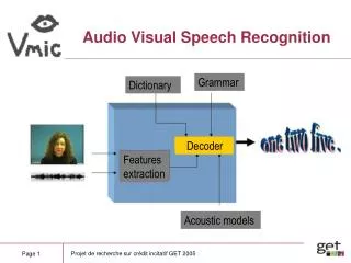
Graphical Methods: Dynamic Bayesian Network • Bayesian Network = A Graph in which • Nodes are Random Variables (RVs) • Edges Represent Dependence • Dynamic Bayesian Network = A BN in which • RVs are repeated once per time step • Example: an HMM is a DBN • Most important RV: the “phonestate” variable qt • Typically qtЄ {Phones} x {1,2,3} • Acoustic features xt and video features yt depend on qt
Example: HMM is a DBN wt-1 wt winct-1 winct ft-1 ft qt-1 qt qinct-1 qinct xt-1 yt-1 xt yt Frame t-1 Frame t • qt is the phonestate, e.g., qtЄ { /w/1, /w/2, /w/3, /n/1, /n/2, … } • wt is the word label at time t, for example, wt Є {“one”, “two”, …} • ft is the position of phone qt within word wt: ftЄ {1st, 2nd, 3rd, …} • qinct Є {0,1} specifies whether ft+1=ft or ft+1=ft+1
Pronunciation Variability • Even when reading phone numbers, talkers “blend” articulations. • For example: “seven eight:” /sevәnet/→ /sevne?/ • As speech gets less formal, pronunciation variability gets worse, e.g., worse in a car than in the lab; worse in conversation than in read speech
A Related Problem: Asynchrony • Audio and Video information are not synchronous • For example: “th” (/q/) in “three” is visible, but not yet audible, because the audio is still silent • Should HMM be in qt=“silence,” or qt=/q/?
A Solution: Two State Variables(Chu and Huang, ICASSP 2000) • Coupled HMM (CHMM): Two parallel HMMs • qt: Audio state (xt: audio observation) • vt: Video state (yt: video observation) • dt=bt-ft: Asynchrony, capped at |dt|<3 wt-1 wt winct-1 winct ft-1 ft qinct-1 qinct qt-1 qt xt-1 xt dt-1 dt bt-1 bt vinct-1 vinct vt-1 vt yt-1 yt Frame t-1 Frame t
word word ind1 ind1 U1 U1 sync1,2 sync1,2 S1 S1 ind2 ind2 U2 U2 sync2,3 sync2,3 S2 S2 ind3 ind3 U3 U3 S3 S3 Asynchrony in Articulatory Phonology(Livescu and Glass, 2004) • It’s not really the AUDIO and VIDEO that are ssynchronous… • It is the LIPS, TONGUE, and GLOTTIS that are asynchronous
Asynchrony in Articulatory Phonology • It’s not really the AUDIO and VIDEO that are ssynchronous… • It is the LIPS, TONGUE, and GLOTTIS that are asynchronous “three,” dictionary form Tongue Dental /q/ Retroflex /r/ Palatal /i/ Glottis Silent Unvoiced Voiced time “three,” casual speech Tongue Dental /q/ Retroflex /r/ Palatal /i/ Glottis Silent Unvoiced Voiced
Asynchrony in Articulatory Phonology • Same mechanism represents pronunciation variability: • “Seven:” /vәn/→ /vn/ if tongue closes before lips open • “Eight:” /et/ → /e?/ if glottis closes before tongue tip closes “seven,” dictionary form: /sevәn/ Lips Fricative /v/ Tongue Fricative /s/ Wide /e/ Closed /n/ Neutral /ә/ time “seven,” casual speech: /sevn/ Lips Fricative /v/ Tongue Fricative /s/ Wide /e/ Closed /n/ Neutral /ә/ time
An Articulatory Feature Model(Hasegawa-Johnson, Livescu, Lal and Saenko, ICPhS 2007) • There is no “phonestate” variable. Instead, we use a vector qt→[lt,tt,gt] • Lipstate variable lt • Tonguestate variable tt • Glotstate variable gt wt-1 wt winct-1 winct lt-1 lt linct-1 linct lt-1 lt dt-1 dt tt-1 tt tinct-1 tinct tt-1 tt et-1 et gt-1 gt ginct-1 ginct gt-1 gt
Experimental Test (Hasegawa-Johnson, Livescu, Lal and Saenko, ICPhS 2007) • Training and test data: CUAVE corpus • Patterson, Gurbuz, Turfecki and Gowdy, ICASSP 2002 • 169 utterances used, 10 digits each, silence between words • Recorded without Audio or Video noise (studio lighting; silent bkgd) • Audio prepared by Kate Saenko at MIT • NOISEX speech babble added at various SNRs • MFCC+d+dd feature vectors, 10ms frames • Video prepared by Amar Subramanya at UW • Feature vector = DCT of lip rectangle • Upsampled from 33ms frames to 10ms frames • Experimental Condition: Train-Test Mismatch • Training on clean data • Audio/video weights tuned on noise-specific dev sets • Language model: uniform (all words equal probability), constrained to have the right number of words per utterance
Experimental Questions(Hasegawa-Johnson, Livescu, Lal and Saenko, ICPhS 2007) • Does Video reduce word error rate? • Does Audio-Video Asynchrony reduce word error rate? • Should asynchrony be represented as • Audio-Video Asynchrony (CHMM), or • Lips-Tongue-Glottis Asynchrony (AFM) • Is it better to use only CHMM, only AFM, or a combination of both methods?
Results, part 1: Should we use video?Answer: YES. Audio-Visual WER < Single-stream WER
Results, part 2: Are Audio and Video be asynchronous?Answer: YES. Async WER < Sync WER.
Results, part 3: Should we use CHMM or AFM?Answer: DOESN’T MATTER! WERs are equal.
Results, part 4: Should we combine systems?Answer: YES. Best is AFM+CH1+CH2 ROVER
Conclusions • Video Feature Extraction: • Manifold discriminant is better than a global discriminant • Audio Feature Extraction: • Beamformer: Delay-and-sum beats Filter-and-sum • Postfilter: Spectral subtraction gives best WER (though MMSE-logSA sounds best) • VAD: Backoff noise estimation works best in this corpus • Audio-Video Fusion: • Video reduces WER in train-test mismatch conditions • Audio and video are asynchronous (CHMM) • Lips, tongue and glottis are asynchronous (AFM) • It doesn’t matter whether you use CHMM or AFM, but... • Best result: combine both representations