Download
1 / 99
1.04k likes | 1.39k Views
Beam Emittance and Beam Profile Monitors by K. Wittenburg –DESY-. Hadron accelerators Wire scanners Residual Gas Ionization (IPM) Residual Gas Scintillation Synchrotron light (Edge effect, wigglers) Scrapers/current (destructive) Emittance preservation. Electron accelerators

E N D
Beam Emittance and Beam Profile Monitorsby K. Wittenburg –DESY-
Hadron accelerators Wire scanners Residual Gas Ionization (IPM) Residual Gas Scintillation Synchrotron light (Edge effect, wigglers) Scrapers/current (destructive) Emittance preservation Electron accelerators Synchrotron light Wire Scanners Scrapers/current (destructive) Laser Wire Scanner Aspect ratio/coupling Transport lines and Linacs Phosphor Screens SEM Grids/Harps OTR Wire scanners (Linacs) Emittance of single shots Idea of this course: Beam Profile monitors use quite a lot of different physical effects to measure the beam size. Many effects on the beam and on the monitor have to be studied before a decision for a type of monitor can be made. In this session we will discuss emittance measurements and we will make some detailed examinations of at least two monitor types to demonstrate the wide range of physics of the profile instruments.
Synchrotron Light Profile Monitor • Introduction • Resolution limits • Small Emittance Measurements • (Proton Synchrotron Radiation Diagnostics)
Synchrotron light profile monitor In electron accelerators the effect of synchrotron radiation (SR) can be used for beam size measurements. In this course we will focus on profile determination, but SR can also be used for bunch length measurements with e.g. streak cameras with a resolution of < 1 ps. From classical electrodynamics the radiated power is given for a momentum change dp/dt and a particle with mass m0 and charge e: For linear accelerators dp/dt = dW/dx. For typical values of dW/dx = 10 - 20 MeV/m the SR is negligible. In circular machines an acceleration perpendicular to the velocity exists mainly in the dipole magnets (field B) with a bending radius r = bgm0c/(eB). The total power of N circulating particles with g = E/m0c2 is than This expression is also valid for a ring having all magnets of the same strength and field-free sections in between. The critical wavelength lc divides the Spectrum of SR in two parts of equal power:
Ψ • Opening angle of SR (1/2 of cone!) for l>>lc(!!!): • with • = E/m0c2 = E [MeV]/0.511 • = 23483 at 12 GeV and • = 52838 at 27 GeV • Path length s: • s = r • r = Bending radius of Dipole J. Flanagan (IPAC2011)
Example HERAe (46 mA circulating electrons at 27 GeV) R = r = 604814.3 mm G = O-L = 6485.5 mm B = L-Z = 1182.3 mm O-S1 = 6216 mm L = Oa-Oi = 1035 mm opening angle (horizontal): tan/2 = d/2/6216 => /2 = arc tan d/2/6216 = 0.85 mrad opening angle (vertikal): (l) = 1/g (l/lc)1/3 Exercise SR1 : Which problems with the setup can be expected?:
Heating of mirror: • total emitted Power per electron: • total Power of 46 mA circulating electrons at 27 GeV (Number of electrons Ne = 6 · 1012) • Ptot = 6 · 106 W • The mirror will get Ptot * Θ / (2 p) = 1600 W (Integral over all wavelength!!!) • Solutions? => mirror is moveable, mirror has to be cooled Material with low Z is nearly not visible for short wavelength => Beryllium Still 100 W on mirror in HERAe not sufficient to prevent image distortion
1. (watercooled) Absorber 2. Do not move the whole mirror into the beam, stop before center
+/- 2 / g = +/- 0,17 mrad „Total“ power within+/- 0,6 mrad
Visible part Fade out ± 2/ gby Absorber Mirrorsize
Grid (yardstick) at point of emission, orbit bumps, … Exercise SR2: What limits the spatial resolution? Diffraction, depth of field, arc, camera => physical Alignment, lenses, mirrors, vibrations => technical How to calibrate the optics?
EQ 1: Diffraction limit (for Object): For normal slit: sDiff = 0.47 * l//2 (horizontal, mirror defines opening angle θ) sDiff 0.47 * l/ (vertikal) Ψ Diffraction:
Ψ Depth of field: EQ 2: depth of field: Vertical: Ddepth L/2 * = s depth Horizontal: Ddepth L/2 * /2 = s depth (mirror defines opening angle θ) L r tanor 2r (/2 + )
Arc: EQ 3: Arc (horizontal): Observation of the beam in the horizontal plane is complicated by the fact that the light is emitted by all points along the arc. The horizontal width of the apparent source is related to the observation angle as: Dxarc = r2/8 = sarc (mirror defines opening angle θ)
Resolution: l not monochromatic ! sDiff = 0.47 * l/ (horizontal) = ??? Depends on wavelength sDiff = 0.47 * l/ (vertikal) = ??? Depends on wavelength sdepth = L/2 * /2 = 440 mm sarc = r 2/8 = 219 mm (horizontal) scamera= schip * G/B = 37 mm Camera (finite pixel size) EQ 4: Camera: image gain = G/B = 5.485 typical resolution of camera CCD chip: schip = 6.7 mm scamera = schip * G/B = 37 mm
Assume: l = 550 nm; (g = E/m0c2) g12 = 2.35 * 104 (E = 12 GeV) g35 = 6.85 * 104 (E = 35 GeV) lc,12 = (4pr)/(3g3) = 0.195 nm at 12 GeV lc,35 = (4pr)/(3g3) = 0.008 nm at 35 GeV opening angle (horizontal): tan/2 = d/2/6216 => /2 = arc tan d/2/6216 = 0.85 mrad opening angle (vertikal): (l) = 1/g (l/lc)1/3 = [(3l)/(4pr)]1/3 = 0.6 mrad (mirror has to be larger than spot size on mirror) => sdiff = 0.47 * l//2 = 304 mm (horizontal) sdiff = 0.47 * l/ = 431 mm (vertical) sdepth = L/2 * /2 = 440 mm sarc = r 2/8 = 219 mm (horizontal) scamera = schip * G/B = 37 mm typical spectral sensitivities from CCD Sensors:
scor = (sdiff 2 + sdepth 2 + sarc2 + scamera 2)1/2 = 579 mm ; (horizontal) scor = (sdiff 2 + sdepth 2 + scamera 2)1/2 = 617 mm ; (vertical) Vertical: scor = [(L/2 * )2 + (0.47 * l/)2]1/2 with L r tan r Horizontal: scor = [(r2/8)2 + (L/2 * /2)2 + (0.47 * l//2)2]1/2 with L r tan r
1) Diffraction: • exact is larger than the Gauss approximation (e.g. 0.79 1.08 mrad at Tristan) • b) For a gaussian beam the diffraction width is sdiff 1/p * l/ • (Ref: ON OPTICAL RESOLUTION OF BEAM SIZE MEASUREMENTS BY MEANS OF SYNCHROTRON RADIATION. By A. Ogata (KEK, Tsukuba). 1991. Published in Nucl.Instrum.Meth.A301:596-598,1991) • => sdiff 1/p * l/exact = 218 mm (exact = 0.8 mrad, l = 550 nm) vertical Not the whole truth: (We measured sometimes a negative emittance???)
2) Depth of field: The formula Rdepth = L/2 * /2 describes the radius of the distribution due to the depth of field effect. It is not gaussian and has long tails. The resolution of an image is probably much better than the formula above. A gaussian approximation with the same integral is shown in the figure below resulting in a width of sdepth = 61 mm.
sdiff = 0.47 * l//2 = 304 mm (horizontal) before: sdiff = 1/p * l/ = 218 mm (vertical) (431 mm) sdepth = L/2 * /2 = 61 mm (440 mm) sarc = r 2/8 = 219 mm (horizontal) scamera = schip * G/B = 37 mm scor = (sdiff 2 + sdepth 2 + sarc2 + scamera 2)1/2 = 381 mm ; (horizontal) (579 mm) scor = (sdiff 2 + sdepth 2 + scamera 2)1/2 = 229 mm ; (vertical) (617 mm) Beam width sbeam = (sfit_measured 2 - scor 2)1/2 svert = 860 mm
Monochromator at shorter wavelength (x-rays, need special optic) • Use optimum readout angle • Polarization - filter • Use x-ray (l < 0.1 nm) • More: • Interferometer • The principle of measurement of the profile • of an object by means of spatial coherency • was first proposed by H.Fizeau and is now • known as the Van Cittert-Zernike theorem. It • is well known that A.A. Michelson measured • the angular dimension (extent) of a star with • this method. • Referenzes • SPATIAL COHERENCY OF THE SYNCHROTRON RADIATION AT THE VISIBLE LIGHT REGION AND ITS APPLICATION FOR THE ELECTRON BEAM PROFILE MEASUREMENT. • By T. Mitsuhashi (KEK, Tsukuba). KEK-PREPRINT-97-56, May 1997. 4pp. Talk given at 17th IEEE Particle Accelerator Conference (PAC 97): Accelerator Science, Technology and Applications, Vancouver, Canada, 12-16 May 1997. • Intensity Interferometer and its application to Beam Diagnostics, ElfimGluskin, ANL, publ. PAC 1991 San Francisco • MEASUREMENT OF SMALL TRANSVERSE BEAM SIZE USING INTERFEROMETRY • T. Mitsuhashi • High Energy Accelerator Research Organisation, Oho, Tsukuba, Ibaraki, 305-0801 Japan • DIPAC 2001 Proceedings - ESRF, Grenoble Exercise SR3: Discuss possible improvements of an SR-monitor:
PETRA III pinhole camera: Ø 18 μm hole in 500 μm thick W plate X-ray Pinhole Camera • „camera obscura“ description of phenomenon already by Aristoteles (384-322 b.C.) in „Problemata“ • most common emittance monitor simple setup limited resolution example: ESRF P.Elleaume, C.Fortgang, C.Penel and E.Tarazona, J.Synchrotron Rad. 2 (1995) , 209 ID-25 X-ray pinhole camera: courtesy of K.Scheidt, ESRF Gero Kube, DESY / MDI
Deff l PETRA III @ 20 keV: • R = 200 μm, R0 = 500 μm, d = 10 μm, l = 1mm • N = 31 • material: beryllium Compound Refractive Lens lens-maker formula: 1/f = 2(n-1) / R concave lens shape strong surface bending R X-ray refraction index : small Z (Be, Al, …) small d many lenses (N=10…300) N Ü Gero Kube, DESY / MDI
X-ray optics γ pinhole optic entrance absorber X-ray optics CCD Monochromator Si (311) Monochromator Si (311) CCD CR lens stack CRL Monitor @ PETRA III (DESY) • PETRA III diagnostics beamline Gero Kube, DESY / MDI
2.) interferometric approach T. Mitsuhashi , Proc. Joint US-CERN-Japan-Russia School of Particle Accelerators, Montreux, 11-20 May 1998 (World Scientific), pp. 399-427. probing spatial coherence of synchrotron radiation visibility: Δn: photon number ΔΦ: photon phase Resolution Improvements extended source point source T. Mitsuhashi, Proc. BIW04, AIP Conf. Proc. 732, pp. 3-18 • resolution limit: uncertainty principle
Interference: ATF (KEK) vertical beam size: courtesy of T.Mitsuhashi, KEK H.Hanyo et al., Proc. of PAC99 (1999), 2143 • smallest result: 4.7 mm with 400nm @ ATF, KEK accuracy ~ 1 mm
Back to an imaging SR-Monitor: Still not the whole truth: Numerical way Includes real electron path, depth of field and diffraction Classical way: approximation
For ∞ mirror size numerical New So far analytical 579 ->381-> 203 mm 617-> 229 -> 138 mm
Comparison SR-monitor vs Wire scanner sv = 542 mm Correction: 617-> 229 -> 138 mm
γ: Lorentz factor ρ: bending radius • spectrum characterized by λc: • large p mass small γ = E/mpc2 Ü Ekin = 20 GeV ρ= 370 m electron λc = 55 mm …4.5 μm proton HERA-p:E = 40…920 GeV large diffraction broadening, expensive optical elements, … Gero Kube, DESY / MDI
consequence: Observation time interval defines spectrum (ωc)
Generation of Frequency Boost sharp cut-off of wavetrain in time domain Ü still requires high beam energies (CERN, Tevatron, HERA) Ü Gero Kube, DESY / MDI
p SyLi Monitor @ HERA (DESY) fringe field of vertical deflecting dipole screen shot : setup : visible light spot for E > 600 GeV dynamics study: additional multiplier signal moving collimators towards the beam time G. Kube et al., Proc. of BIW06 (2006), Batavia, Illinois, p.374 Gero Kube, DESY / MDI
Superconducting Accelerating Structures Collimator Undulators dispersive section information about energy distribution (and more…) Bunch Compressor Bunch Compressor FEL diagnostics bypass 5 MeV 130 MeV 450 MeV 400 … 1000 MeV 250 m Energy Monitor @ FLASH (DESY) SR based profile diagnostics in bunch compressor stability : single bunch Ch.Gerth, Proc. of DIPAC07 (2007), Venice, p.150 Gero Kube, DESY / MDI
Wire Scanners Introduction Conventional wire scanners with thin solid wires (conventional compared with new techniques using, for example, Lasers) are widely used for beam size measurements in particle accelerators. • Their advantages: • Resolution of down to 1 mm • Trusty, reliable • Direct
0.1 micron position resolution is possible Potentiometer
CERN/DESY 1990-2007 FLASH: 2002 - now Speed: 0 - 1 m/s Scanning area: approx. 10 cm Wire material: Carbon/Quartz Wire diameter: 7 microns 50 mm at Flash Signal: shower 1 micron resolution
Projected angular distribution could be approximated by Gaussian with a width given by d’ = 1.510-3 cm – the thickness of the target, X0=12.3 cm – quartz-wire radiation length, x/X0 = 1.2210-4 It is corresponding to: mean 3.010-6 rad for electron momentum of 30GeV/c. Scattered particles will arrive vacuum chamber of radius R = 2 cm at: What to do? Where one should locate the Scintillator?
Protons at 920 GeV/c Electrons at 30 GeV/c Wire position: -100cm Counter: 29 cm Monte Carlo simulations for finding best location of scintillators Wire scanner: -8.1 m Counter: 20 m Simulation includes all magnetic fields as well as all elastic and inelastic scattering cross sections
Wire Scanner at low energies Wire scanners in low energy accelerators P. Elmfos ar. Al.; NIM A 396
Wire Scanner at low energies • 2) Secondary electron emission (SEM) . • This method is often used at low energy beams where the scattered particles cannot penetrate the vacuum pipe wall (below pion threshold). • Avoid cross talk of wires • In this low energy regime the hadron beam particles stop in the wire, so that the signal is a composition of the stopped charge (in case of H-: proton and electrons) and the secondary emission coefficient. Therefore the polarity of the signal may change, depending on the beam energy and particle type (true also for grids!). (stripping) M. A. Plum, et al, SNS LINAC WIRE SCANNER SYSTEM, Signal Levels and Accuracy; LINAC2002
Wire scanner’s limitations are? 1. The smallest measurable beam size is limited by the finite wire diameter of a few microns, 2. Higher Order Modes may couple to conductive wires and can destroy them, 3. High beam intensities combined with small beam sizes will destroy the wire due to the high heat load. 4. Emittance blow up
Limitations: 1. Wire size The smallest achievable wires have a diameter of about 5-6 mm. An example of the error in the beam width determination is shown for a 36 mm wire. Influence of the wire diameter on the measured beam width. (All figures from: Q. King; Analysis of the Influence of Fibre Diameter on Wirescanner Beam Profile Measurements, SPS-ABM-TM/Note/8802 (1988))
Limitations: 2. Higher Order modes An early observation (1972 DORIS) with wire scanners in electron accelerators was, that the wire was always broken, even without moving the scanner into the beam. An explanation was that Higher Order Modes (HOM) were coupled into the cavity of the vacuum chamber extension housing the wire scanner fork. The wire absorbs part of the RF which led to strong RF heating. Exercise WIRE1: 1) Discuss methods of proving this behavior. • Methods: • Measurement of wire resistivity • Measurement of thermo-ionic emission • Optical observation of glowing wire • Measurement of RF coupling in Laboratory with spectrum analyzer
Measurement of wire resistivity The wire resistivity will change depending on the temperature of the wire, even without scanning. Here: 8 mm Carbon wire (from OBSERVATION OF THERMAL EFFECTS ON THE LEP WIRE SCANNERS. By J. Camas, C. Fischer, J.J. Gras, R. Jung, J. Koopman (CERN). CERN-SL-95-20-BI, May 1995. 4pp. Presented at the 16th Particle Accelerator Conference - PAC 95, Dallas, TX, USA, 1 - 5 May 1995. Published in IEEE PAC 1995:2649-2651)