Download
1 / 21
230 likes | 427 Views
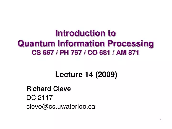
Introduction to Quantum Information Processing CS 667 / PH 767 / CO 681 / AM 871. Lecture 14 (2009). Richard Cleve DC 2117 cleve@cs.uwaterloo.ca. Bloch sphere for qubits. Bloch sphere for qubits (1). Consider the set of all 2x2 density matrices .

E N D
Introduction to Quantum Information ProcessingCS 667 / PH 767 / CO 681 / AM 871 Lecture 14 (2009) Richard Cleve DC 2117 cleve@cs.uwaterloo.ca
Bloch sphere for qubits (1) Consider the set of all 2x2 density matrices They have a nice representation in terms of the Pauli matrices: Note that these matrices—combined with I—form a basis for the vector space of all 2x2 matrices We will express density matrices in this basis Note that the coefficient of I is ½, since X, Y, Y are traceless
Bloch sphere for qubits (2) We will express First consider the case of pure states , where, without loss of generality, =cos()0 +e2isin()1 (,R) Therefore cz= cos(2),cx= cos(2)sin(2),cy= sin(2)sin(2) These are polar coordinates of a unit vector (cx ,cy ,cz)R3
0 –i + – +i 1 + = 0 +1 – = 0 – 1 +i = 0 +i1 –i = 0 –i1 Bloch sphere for qubits (3) Note that orthogonal corresponds to antipodal here Pure states are on the surface, and mixed states are inside (being weighted averages of pure states)
0 with prob. ½ 1 with prob. ½ 0 with prob. cos2(/8) 1 with prob. sin2(/8) 0 with prob. ½ 1 with prob. ½ 1 + 0 0 with prob. ½ 0 +1 with prob. ½ 0 Distinguishing mixed states (1) What’s the best distinguishing strategy between these two mixed states? 1 also arises from this orthogonal mixture: … as does 2 from:
Distinguishing mixed states (2) We’ve effectively found an orthonormal basis 0,1 in which both density matrices are diagonal: 1 1 + 0 Rotating 0,1to 0, 1the scenario can now be examined using classical probability theory: 0 Distinguish between two classical coins, whose probabilities of “heads” are cos2(/8)and ½ respectively (details: exercise) Question: what do we do if we aren’t so lucky to get two density matrices that are simultaneously diagonalizable?
General quantum operations (1) Also known as: “quantum channels” “completely positive trace preserving maps”, “admissible operations” LetA1, A2 , …, Am be matrices satisfying Then the mapping is a general quantum op Note:A1, A2 , …, Am do not have to be square matrices Example 1 (unitary op): applying U to yieldsUU†
After looking at the outcome, becomes 00 with prob. ||2 11 with prob. ||2 General quantum operations (2) Example 2 (decoherence):letA0 =00andA1 =11 This quantum op maps to 0000 + 1111 For ψ =0 +1, Corresponds to measuring “without looking at the outcome”
General quantum operations (3) Example 3 (discarding the second of two qubits): LetA0 =I0andA1 =I1 States of the form (product states) become State becomes Note 1: it’s the same density matrix as for ((½, 0), (½, 1)) Note 2: the operation is called the partial traceTr2
More about the partial trace Two quantum registers in states and (resp.) are independent when the combined system is in state = If the 2nd register is discarded, state of the 1st register remains In general, the state of a two-register system may not be of the form (it may contain entanglement or correlations) The partial trace Tr2gives the effective state of the first register For d-dimensional registers, Tr2 is defined with respect to the operators Ak =Ik, where0, 1, …, d1 can be any orthonormal basis The partial trace Tr2 ,can also be characterized as the unique linear operator satisfying the identity Tr2( )=
Partial trace continued For 2-qubit systems, the partial trace is explicitly and
General quantum operations (4) Example 4 (adding an extra qubit): Just one operatorA0 =I0 States of the form become 00 More generally, to add a register in state , use the operator A0=I
POVM measurements (POVM = Positive Operator Valued Measre)
Corresponding POVM measurement is a stochastic operation on that, with probability , produces outcome: j (classical information) (the collapsed quantum state) POVM measurements (1) LetA1, A2 , …, Am be matrices satisfying Example 1:Aj = jj (orthogonal projectors) This reduces to our previously defined measurements …
POVM measurements (2) When Aj = jj are orthogonal projectors and = , = Trjjjj = jjjj = j2 Moreover,
DefineA0 =2/300 A1=2/311 A2=2/322 POVM measurements (3) Example 3 (trine state“measurent”): Let 0 = 0, 1 =1/20 + 3/21, 2 =1/20 3/21 Then If the input itself is an unknown trine state, kk, then the probability that classical outcome is k is 2/3 = 0.6666…
POVM measurements (4) Often POVMs arise in contexts where we only care about the classical part of the outcome (not the residual quantum state) The probability of outcome j is Simplified definition for POVM measurements: LetE1, E2 , …, Em be positive definite and such that The probability of outcome j is This is usually the way POVM measurements are defined
“Mother of all operations” LetA1,1, A1,2 , …, A1,m1 satisfy A2,1, A2,2 , …, A2,m2 Ak,1, Ak,2 , …, Ak,mk Then there is a quantum operation that, on input , produces with probability the state: j (classical information) (the collapsed quantum state)