Download
1 / 28
280 likes | 481 Views
Introduction to Quantum Information Processing QIC 710 / CS 667 / PH 767 / CO 681 / AM 871. Lectures 17-19 (2011). Richard Cleve DC 2117 cleve@cs.uwaterloo.ca. Complexity class NP. Complexity classes. Recall:.

E N D
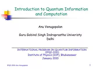
Introduction to Quantum Information ProcessingQIC 710 / CS 667 / PH 767 / CO 681 / AM 871 Lectures 17-19 (2011) Richard Cleve DC 2117 cleve@cs.uwaterloo.ca
Complexity classes Recall: • P (polynomial time):problems solved by O(nc)-size classical circuits (decision problems and uniform circuit families) • BPP (bounded error probabilistic polynomial time): problems solved by O(nc)-size probabilistic circuits that err with probability ¼ • BQP (bounded error quantum polynomial time):problems solved by O(nc)-size quantum circuits that err with probability ¼ • PSPACE (polynomial space): problems solved by algorithms that use O(nc) memory.
Summary of previous containments P BPP BQP PSPACE EXP EXP We now consider further structure between Pand PSPACE PSPACE BQP Technically, we will restrict our attention to languages (i.e. {0,1}-valued problems) BPP P Many problems of interest can be cast in terms of languages For example, we could define FACTORING= {(x,y) : 2 zy, such thatzdividesx}
is satisfiable iff there exists such that NP Define NP (non-deterministic polynomial time)as the class of languages whose positive instances have “witnesses” that can be verified in polynomial time Example: Let 3-CNF-SAT be the language consisting of all 3-CNF formulas that are satisfiable 3-CNF formula: No sub-exponential-time algorithm is known for 3-CNF-SAT But poly-time verifiable witnesses exist (namely, b1, ..., bn)
1 output bit Λ Λ 0 Λ Λ Λ 1 Λ Λ Λ Λ 1 Λ Λ 0 Λ Λ Λ Other “logic” problems in NP • k-DNF-SAT: • CIRCUIT-SAT: But, unlike with k-CNF-SAT, this one is known to be in P All known algorithms exponential-time
“Graph theory” problems in NP • k-COLOR:does G have a k-coloring? • k-CLIQUE:does G have a clique of size k? • HAM-PATH:does G have a Hamiltonian path? • EUL-PATH:does G have an Eulerian path?
“Arithmetic” problems in NP • FACTORING={(x,y) : 2 zy, such thatzdividesx} • SUBSET-SUM:given integers x1, x2 , ..., xn, y, do there exist i1, i2 , ..., ik {1, 2,... , n} such that xi1+xi2+ ... +xik= y? • INTEGER-LINEAR-PROGRAMMING:linear programming where one seeks an integer-valued solution(its existence)
P vs. NP All of the aforementioned problems have the property that they reduce to 3-CNF-SAT, in the sense that a polynomial-time algorithm for 3-CNF-SAT can be converted into a poly-time algorithm for the problem Example: algorithm for 3-COLOR algorithm for 3-CNF-SAT If a polynomial-time algorithm is discovered for 3-CNF-SAT then a polynomial-time algorithm for 3-COLOR follows And this holds for any problem XNP
P vs. NP For any problem XNP algorithm for X algorithm for 3-CNF-SAT A problem that has this property is said to be NP-hard Polynomial-time algorithm any NP-Hard problem implies P=NP NP-hard problems: 3-CNF-SAT, CIRCUIT-SAT, 3-COLOR , k-CLIQUE, HAM-PATH, SUBSET-SUM, INT-LIN-PROG, … Some problems in P: k-DNF-SAT, 2-COLOR, 3-CLIQUE, EUL-PATH,...
PSPACE NP co-NP 3-CNF-SAT FACTORING P FACTORING vs. NP Is FACTORINGNP-hard too? If so, then every problem in NP is solvable by a poly-time quantum algorithm! But FACTORING has not been shown to be NP-hard Moreover, there is “evidence” that it is not NP-hard: FACTORING NPco-NP If FACTORING is NP-hard then NP=co-NP
FACTORING vs.co-NP FACTORING= {(x,y) : 2 zy, s.t. zdividesx} co-NP: languages whose negative instances have “witnesses” that can be verified in poly-time PSPACE NP co-NP Question: what is a good witness for the negative instances? FACTORING P Answer: the prime factorization p1, p2, ..., pm of x will work Can verify primality and compare p1, p2, ..., pm with y, all in poly-time
x1 x1 Uf xn xn y y f(x1,...,xn) Quantum search problem Given: a black box computing f : {0,1}n {0,1} Goal: determine if f is satisfiable (if x {0,1}n s.t. f(x) = 1) In positive instances, it makes sense to also find such a satisfying assignment x Classically, using probabilistic procedures, order 2n queries are necessary to succeed—even with probability ¾ (say) Grover’s quantum algorithm that makes only O(2n) queries Query: [Grover ’96]
PSPACE NP co-NP 3-CNF-SAT FACTORING P Applications of quantum search The function f could be realized as a 3-CNF formula: Alternatively, the search could be for a certificate for any problem in NP The resulting quantum algorithms appear to be quadratically more efficient than the best classical algorithms known* Subtlety in that the search space might have to be redefined to achieve this
reflection 2 reflection 1 Prelude to Grover’s algorithm: two reflections = a rotation Consider two lines with intersection angle : 2 2 1 1 Net effect: rotation by angle 2, regardless of starting vector
H X X X H X X X H x1 x1 x1 x1 H U0 Uf xn xn xn xn y y y f(x1,...,xn) y [x=0...0] Grover’s algorithm: description I Basic operations used: Uf x = (1) f(x)x Implementation? U0x = (1)[x=0...0]x Hadamard
iteration 2 ... iteration 1 0 U0 Uf Uf U0 H H H H H 0 Grover’s algorithm: description II • construct state H0...0 • repeatktimes: • apply HU0HUfto state • 3. measure state, to get x{0,1}n, and check if f(x)=1 (The setting of k will be determined later)
Let and A B Grover’s algorithm: analysis I Let A={x{0,1}n : f(x) = 1} and B={x{0,1}n : f(x) = 0} and N= 2n and a=|A| and b=|B| Consider the space spanned by AandB goal is to get close to this state H0...0 Interesting case: a << N
A B Grover’s algorithm: analysis II Algorithm: (HU0HUf)kH0...0 H0...0 Observation: Uf is a reflection about B: UfA =AandUfB =B Question: what is HU0H ? U0 is a reflection about H0...0 Partial proof: HU0HH0...0=HU00...0 =H(0...0) =H0...0
A Since HU0HUf is a composition of two reflections, it is a rotation by 2, wheresin()=a/N a/N More generally, it suffices to set k (/4)N/a B Grover’s algorithm: analysis III Algorithm: (HU0HUf)kH0...0 2 2 2 H0...0 2 When a = 1, we want (2k+1)(1/N) /2 , so k (/4)N Question: what if a is not known in advance?
Unknown number of solutions 1 solution 2 solutions 3 solutions 1 success probability 0 number of iterations 100 solutions 4 solutions 6 solutions success probability very close to zero! √N/2 Choose a randomk in the range to get success probability >0.43
Optimality of Grover’s algorithm
U0 f U1 f U2 f f U3 f Uk |x (1)f(x)|x Assume queries are of the form Optimality of Grover’s algorithm I Theorem: any quantum search algorithm for f: {0,1}n {0,1}must make (2n) queries to f (if f is used as a black-box) Proof (of a slightly simplified version): and that a k-query algorithm is of the form |0...0 where U0, U1, U2, ..., Uk, are arbitrary unitary operations
U0 U0 fr I U1 U1 I fr U2 U2 fr I U3 U3 fr I Uk Uk |0 |0 Optimality of Grover’s algorithm II Define fr: {0,1}n {0,1} as fr (x) = 1 iff x = r Consider |ψr,k versus |ψr,0 We’ll show that, averaging over all r {0,1}n, |||ψr,k |ψr,0|| 2k/2n
|ψr,i U0 I U1 I U2 fr U3 fr Uk i ki |0 Note that |ψr,k |ψr,0 =(|ψr,k |ψr,k1)+ (|ψr,k1 |ψr,k2)+ ... +(|ψr,1 |ψr,0) which implies |||ψr,k |ψr,0|| |||ψr,k |ψr,k1|| + ... + |||ψr,1 |ψr,0|| Optimality of Grover’s algorithm III Consider
query i query i+1 |ψr,i query i query i+1 U0 U0 I I U1 U1 I I U2 U2 I fr U3 U3 fr fr Uk Uk |ψr,i-1 |0 |0 Therefore, |||ψr,k |ψr,0|| Optimality of Grover’s algorithm IV |||ψr,i |ψr,i-1|| =|2i,r|,since query only negates|r
Optimality of Grover’s algorithm V Now, averaging over all r {0,1}n, (By Cauchy-Schwarz) Therefore, for somer{0,1}n, the number of queries k must be (2n), in order to distinguish fr from the all-zero function This completes the proof