Download

1 / 40
400 likes | 513 Views
Algorithmic High-Dimensional Geometry 2. Alex Andoni ( Microsoft Research SVC). The NNS prism. High dimensional geometry. dimension reduction. NNS. space partitions. small dimension. embedding. sketching. …. Small Dimension. What if is small?. Can solve approximate NNS with

E N D
Algorithmic High-Dimensional Geometry 2 Alex Andoni (Microsoft Research SVC)
The NNS prism High dimensional geometry dimension reduction NNS space partitions small dimension embedding sketching …
What if is small? • Can solve approximate NNS with • space • query time • [AMNSW’98,…] • OK, if say ! • Usually, is not small…
“effectively” What if is small? • Eg: • -dimensional subspace of , with • Obviously, extract subspace and solve NNS there! • Not a robust definition… • More robust definitions: • KR-dimension [KR’02] • Doubling dimension [Assouad’83, Cla’99, GKL’03, KL’04] • Smooth manifold [BW’06, Cla’08] • other [CNBYM’01, FK97, IN’07, Cla’06…]
Doubling dimension • Definition: pointset has doubling dimensionif: • for any point , radius , consider ball of points within distance of • can cover by balls , … • Sanity check: • -dimensional subspace has • npoints always have dimension at most • Can be defined for any metric space! balls to cover
NNS for small doubling dimension • Euclidean space[Indyk-Naor’07] • JL into dimension “works” ! • Contractionof any pair happens with very small probability • Expansion of some pair happens with constant probability • Good enough for NNS! • Arbitrary metric • Navigating nets/cover trees [Krauthgamer-Lee’04, Har-Peled-Mendel’05, Beygelzimer-Kakade-Langford’06,…] • Algorithm: • A data-dependent tree: recursive space partition using balls • At query , follow all paths that intersect with the ball
General Theory: embeddings • General motivation: given distance (metric) , solve a computational problem under Hamming distance Compute distance between two points Euclidean distance (ℓ2) Nearest Neighbor Search Diameter/Close-pair of set S Edit distance between two strings Earth-Mover (transportation) Distance Clustering, MST, etc Reduce problem <under hard metric> to <under simpler metric>
Embeddings: landscape • Definition: an embedding is a map of a metric into a host metric such that for any : where is the distortion (approximation) of the embedding . • Embeddings come in all shapes and colors: • Source/host spaces • Distortion • Can be randomized: withprobability • Time to compute • Types of embeddings: • From norm to the same norm but of lower dimension (dimension reduction) • From one norm () into another norm () • From non-norms (edit distance, Earth-Mover Distance) into a norm () • From given finite metric (shortest path on a planar graph) into a norm () • not a metric but a computational procedure sketches
Earth-Mover Distance • Definition: • Given two sets of points in a metric space • = min cost bipartite matching between and • Which metric space? • Can be plane, … • Applications in image vision Images courtesy of Kristen Grauman
Embedding EMD into • At least as hard as • Theorem [Cha02, IT03]: Can embed EMD over into with distortion . Time to embed a set of points: . • Consequences: • Nearest Neighbor Search: approximation with space, and query time. • Computation: approximation in time • Best known: approximation in time [SA’12] • The higher-dimensional variant is still fastest via embedding [AIK’08]
High level embedding • Sets of size in box • Embedding of set : • take a quad-tree • randomly shift it • Each cell gives a coordinate: =#points in the cell • Need to prove 0 0 0 0 1 1 0 2 2 2 1 2 1 0 2 0 0 0 1 0 …2210… 0002…0011…0100…0000… …1202… 0100…0011…0000…1100…
Main Approach • Idea: decompose EMD over []2 into EMDs over smaller grids • Recursively reduce to =O(1) ≈ +
EMD over small grid • Suppose =3 • f(A) has nine coordinates, counting # points in each joint • f(A)=(2,1,1,0,0,0,1,0,0) • f(B)=(1,1,0,0,2,0,0,0,1) • Gives O(1) distortion
Decomposition Lemma [I07] • For randomly-shifted cut-grid G of side length k, we have: • EEMD(A,B) ≤ EEMDk(A1, B1) + EEMDk(A2,B2)+… +k*EEMD/k(AG, BG) • EEMD(A,B) [ EEMDk(A1, B1) + EEMDk(A2,B2)+… ] • EEMD(A,B) [k*EEMD/k(AG, BG) ] • The distortion will follow by applying the lemma recursively to (AG,BG) lower bound on cost upper bound k /k
Part 1: lower bound • For a randomly-shifted cut-grid G of side length k, we have: • EEMD(A,B) ≤ EEMDk(A1, B1) + EEMDk(A2,B2)+… +k*EEMD/k(AG, BG) • Extract a matching from the matchings on right-hand side • For each aA, with aAi, it is either: • matched in EEMD(Ai,Bi) to some bBi • or aAi\Bi, and it is matched in EEMD(AG,BG) to some bBj • Match cost in 2nd case: • Move a to center () • paid by EEMD(Ai,Bi) • Move from cell i to cell j • paid by EEMD(AG,BG) k /k
Parts 2 & 3: upper bound • For a randomly-shifted cut-grid G of side length k, we have: • EEMD(A,B) [ EEMDk(A1, B1) + EEMDk(A2,B2)+… ] • EEMD(A,B) [ k*EEMD/k(AG, BG) ] • Fix a matching minimizing EEMD(A,B) • Will construct matchings for each EEMD on RHS • Uncut pairs (a,b) are matched in respective (Ai,Bi) • Cut pairs (a,b) are matched • in (AG,BG) • and remain unmatched in their mini-grids
Part 2: Cost? • EEMD(A,B) [ ∑iEEMDk(Ai, Bi)] • Uncut pairs (a,b) are matched in respective (Ai,Bi) • Contribute a total ≤ EEMD (A,B) • Consider a cut pair (a,b)at distance • Contribute ≤ 2k to ∑iEEMDk(Ai, Bi) • Pr[(a,b) cut] = • Expected contribution ≤ Pr[(a,b) cut] • In total, contribute EEMD(A,B) k dx
Wrap-up of EMD Embedding • In the end, obtain that • EMD(A,B) sum of EMDs of smaller grids in expectation • Repeat times to get to grid • approximation it total!
Embeddings of various metrics into edit( banana , ananas ) = 2 edit(1234567, 7123456) = 2
Non-embeddability proofs • Via Poincaré-type inequalities… • [Enflo’69]: embedding into (any dimension) must incur distortion • Proof [Khot-Naor’05] • Suppose is the embedding of into • Two distributions over pairs of points : • C: for random and index • F:are random • Two steps: • (short diagonals) • Implies lower bound!
Other good host spaces? • What is “good”: • is algorithmically tractable • is rich (can embed into it) ,etc ??? sq-ℓ2=real space with distance: ||x-y||22 sq-ℓ2, hosts with very good LSH (lower bounds via communication complexity) ̃ [AK’07] [AK’07] [AIK’08]
The story • [Mat96]:Can embed any metric on points into • Theorem [I’98]: NNS for with • approximation • space, • query time • Dimension is an issue though… • Smaller dimension? • Possible for some: Hausdorff,… [FCI99] • But, not possible even for [JL01]
Other good host spaces? • What is “good”: • algorithmically tractable • rich (can embed into it) • But: combination sometimes works! ,etc
d1 d1 … … d∞,1 d∞,1 α Meet our new host d1 [A-Indyk-Krauthgamer’09] … • Iterated product space β d∞,1 d22,∞,1 γ
Why ? edit distance between permutations ED(1234567, 7123456) = 2 [Indyk’02, A-Indyk-Krauthgamer’09] • Because we can… • Embedding: …embed Ulam into with constantdistortion • dimensions = length of the string • NNS: Any t-iterated product space has NNS on n points with • approximation • near-linear space and sublinear time • Corollary: NNS for Ulam with approx. • Better than via each component separately! Rich Algorithmically tractable
Computational view x y • Arbitrary computation • Cons: • No/little structure (e.g., not metric) • Pros: • More expressability: • may achieve better distortion (approximation) • smaller “dimension” • Sketch: “functional compression scheme” • for estimating distances • almost all lossy (distortion or more) and randomized F F(x) F(y)
Why? • 1) Beyond embeddings: • can more do if “embed” into computational space • 2) A waypoint to get embeddings: • computational perspective can give actual embeddings • 3) Connection to informational/computational notions • communication complexity
Beyond Embeddings: • “Dimension reduction” in ! • Lemma [I00]: exists linear , and • where • achieves: for any , with probability : • Wherewith each distributed from Cauchy distribution (-stable distribution) • While does not have expectation, it has median!
Waypoint to get embeddings • Embedding of Ulam metric into was obtained via “geometrization” of an algorithm/characterization: • sublinear (local) algorithms: property testing & streaming [EKKRV98, ACCL04, GJKK07, GG07, EJ08] edit(X,Y) sum of squares (sq-ℓ2) max (ℓ∞) sum (ℓ1) X Y
Ulam: algorithmic characterization [Ailon-Chazelle-Commandur-Lu’04, Gopalan-Jayram- Krauthgamer-Kumar’07, A-Indyk-Krauthgamer’09] E.g., a=5; K=4 • Lemma: Ulam(x,y) approximately equals the number of “faulty” characters a satisfying: • there exists K≥1 (prefix-length) s.t. • the set of K characters preceding a in xdiffers muchfrom the set of K characters preceding a in y X[5;4] 123456789 x= y= 123467895 Y[5;4]
… Connection to communication complexity • Enter the world of Alice and Bob… Communication complexity model: • Two-party protocol • Shared randomness • Promise (gap) version • c = approximation ratio • CC = min. # bits to decide (for 90% success) shared randomness CC bits Sketching model: • Referee decides based on sketch(x), sketch(y) • SK= min. sketch size to decide Fact:SK ≥ CC sketch() sketch() Referee decide whether: or
Communication Complexity • VERY rich theory [Yao’79, KN’97,…] • Some notable examples: • are sketchable with bits! [AMS’96,KOR’98] • hence also everything than embeds into it! • is tight [IW’03,W’04, BJKS’08,CR’12] • requires bits [BJKS’02] • Coresets: sketches of sets of points for geometric problems [AHV04…] • Connection to NNS: • [KOR’98]: if sketch size is , then NNS with space and one memory lookup! • From the perspective of NNS lower bounds, communication complexity closer to ground truth • Question: do non-embeddability result say something about non-sketchability? • also Poincaré-type inequalities… [AK07,AJP’10] • Connections to streaming: see Graham Cormode’s lecture
High dimensional geometry ???
Closest Pair • Problem: n points in d-dimensional Hamming space, which are random except a planted pair at distance ½- • Solution 1: build NNS and query times • LSH-type algowould give ~[PRR89,IM98,D08] • Theorem [Valiant’12]: time p1 p1 p1+p2 p2 p2 = M Find max entry of MMt using subcubic MM algorithms pn pn
What I didn’t talk about: • Too many things to mention • Includes embedding of fixed finite metric into simpler/more-structured spaces like • Tiny sample among them: • [LLR94]: introduced metric embeddings to TCS. E.g. showed can use [Bou85] to solve sparsest cut problem with approximation • [Bou85]: Arbitrary metric on points into , with distortion • [Rao99]: embedding planar graphs into , with distortion • [ARV04,ALN05]: sparsest cut problem with approximation • [KMS98,…]: space partition for rounding SDPs for coloring • Lots others… • A list of open questions in embedding theory • Edited by JiříMatoušek + AssafNaor: • http://kam.mff.cuni.cz/~matousek/metrop.ps
High dimensional geometry via NNS prism High dimensional geometry dimension reduction NNS space partitions small dimension embedding sketching +++